Permformance
Introduction
Optimizing code to make it run faster is an iterative process:
| Step | What to do | Me |
|---|---|---|
| 01 | Find the biggest bottleneck | the slowest part of your code |
| 02 | Try to eliminate it | you may not succeed but that’s ok |
| 03 | Repeat until your code is “fast enough” | This sounds easy, but it’s not |

Instead of relying on your intuition, you should profile your code:
use realistic inputs and measure the run-time of each individual operation.
Only once you’ve identified the most important bottlenecks can you attempt to eliminate them.
Prerequisites
lineprof package helps in measuring the performance of R
code.
# devtools::install_github("hadley/lineprof")
# install.packages("profvis")
library("profvis")
Measuring performance
To speed up computations it can be usefull to
check how much time R spends in its calculations.
| Function | Action |
|---|---|
Rprof() |
enables profiling of the execution of R expressions |
summaryRprof() |
shows the amount of time used by different R functions. |
library(lattice)

data(melanoma)

melanoma=melanoma[1:20,]

head(melanoma)
## year incidence
## 1 1936 0.9
## 2 1937 0.8
## 3 1938 0.8
## 4 1939 1.3
## 5 1940 1.4
## 6 1941 1.2Let’s fit X as regression model on incidence and be y
the years.
Use the least squares formula to approximate solution of
this overdetermined system.
Least squares means that the overall solution minimizes the sum of the squares of the errors made in the results of every single equation.
Text book formula for least squares estimate:
\[[ t(X)*X ]*t(X)*y\]
 # let be (X,y) our overdetermined system
#     or a system of linear equations.

X <- model.matrix(~incidence+I(incidence^2)+I(incidence^3),
                                    data=melanoma)

y <- melanoma$year

lsfit1 <- function(X, y) {
  # solve() solves the equation a %*% x = b
  solve(t(X) %*% X) %*% t(X) %*% y
}

Rprof() # Function that I wanna profile ________

for (ii in 1:10000) lsfit1(X,y)

Rprof(NULL) # close profiling ________

rr<-summaryRprof()

## timings sorted by ‘total’ time
# time  = times in seconds spent executing code in that function
# pct   = percentages of the total time spent executing code in that function

rr$by.total
## total.time total.pct self.time self.pct
## "eval_with_user_handlers" 0.26 100.00 0.02 7.69
## "block_exec" 0.26 100.00 0.00 0.00
## "call_block" 0.26 100.00 0.00 0.00
## "eng_r" 0.26 100.00 0.00 0.00
## "evaluate_call" 0.26 100.00 0.00 0.00
## "evaluate::evaluate" 0.26 100.00 0.00 0.00
## "evaluate" 0.26 100.00 0.00 0.00
## "FUN" 0.26 100.00 0.00 0.00
## "generator$render" 0.26 100.00 0.00 0.00
## "handle" 0.26 100.00 0.00 0.00
## "in_dir" 0.26 100.00 0.00 0.00
## "in_input_dir" 0.26 100.00 0.00 0.00
## "knitr::knit" 0.26 100.00 0.00 0.00
## "lapply" 0.26 100.00 0.00 0.00
## "process_file" 0.26 100.00 0.00 0.00
## "process_group.block" 0.26 100.00 0.00 0.00
## "process_group" 0.26 100.00 0.00 0.00
## "render_one" 0.26 100.00 0.00 0.00
## "rmarkdown::render_site" 0.26 100.00 0.00 0.00
## "rmarkdown::render" 0.26 100.00 0.00 0.00
## "sapply" 0.26 100.00 0.00 0.00
## "suppressMessages" 0.26 100.00 0.00 0.00
## "timing_fn" 0.26 100.00 0.00 0.00
## "withCallingHandlers" 0.26 100.00 0.00 0.00
## "withVisible" 0.26 100.00 0.00 0.00
## "eval" 0.24 92.31 0.00 0.00
## "lsfit1" 0.24 92.31 0.00 0.00
## "solve" 0.16 61.54 0.00 0.00
## "solve.default" 0.10 38.46 0.04 15.38
## "t.default" 0.08 30.77 0.08 30.77
## "t" 0.08 30.77 0.00 0.00
## "%*%" 0.04 15.38 0.04 15.38
## "colnames<-" 0.02 7.69 0.02 7.69
## "diag" 0.02 7.69 0.02 7.69
## "findCenvVar" 0.02 7.69 0.02 7.69
## "lazyLoadDBfetch" 0.02 7.69 0.02 7.69
## "cmp" 0.02 7.69 0.00 0.00
## "cmpBuiltinArgs" 0.02 7.69 0.00 0.00
## "cmpCall" 0.02 7.69 0.00 0.00
## "cmpfun" 0.02 7.69 0.00 0.00
## "compiler:::tryCmpfun" 0.02 7.69 0.00 0.00
## "doTryCatch" 0.02 7.69 0.00 0.00
## "findLocVar" 0.02 7.69 0.00 0.00
## "genCode" 0.02 7.69 0.00 0.00
## "h" 0.02 7.69 0.00 0.00
## "tryCatch" 0.02 7.69 0.00 0.00
## "tryCatchList" 0.02 7.69 0.00 0.00
## "tryCatchOne" 0.02 7.69 0.00 0.00
## "tryInline" 0.02 7.69 0.00 0.00Limitations
There are some other limitations to profiling:
Profiling does not extend to C code. You can see if your R code calls C/C++ code but not what functions are called inside of your C/C++ code. Unfortunately, tools for profiling compiled code are beyond the scope of this book (i.e., I have no idea how to do it).
Similarly, you can’t see what’s going on inside primitive functions or byte code compiled code.
What to do?
Once you’ve used profiling to identify a bottleneck, you need to make it faster. The following sections introduce you to a number of techniques.
- Look for existing solutions.
- Do less work.
- Vectorise.
- Parallelise.
- Avoid copies.
- Byte-code compile.
A final technique is to:
- rewrite in a faster language, like C++.
That’s a big topic and is covered in Rcpp.
Code organisation
There are two traps that are easy to fall into when trying to make your code faster:
- Writing faster but incorrect code.
- Writing code that you think is faster, but is actually no better.
When tackling a bottleneck, you’re likely to come up with multiple approaches.
Write a function for each approach, encapsulating all relevant behaviour.
This makes it easier to check that each approach returns the correct result and to time how long it takes to run.
mean1 <- function(x) mean(x)
mean2 <- function(x) sum(x) / length(x)
Use this test case to quickly check that all variants return the same result.
An easy way to do so is with stopifnot() and
all.equal().
x <- runif(100)
stopifnot( all.equal(mean1(x), mean2(x)) )
Finally, use the microbenchmark package to compare how
long each variation takes to run.
library(microbenchmark)

microbenchmark(
  mean1(x),
  mean2(x)
  ,unit = "us"
)
## Unit: microseconds
## expr min lq mean median uq max neval cld
## mean1(x) 15.793 16.292 24.22022 16.3755 16.501 656.417 100 a
## mean2(x) 12.167 12.584 26.61483 12.6670 12.751 1342.584 100 aDo as little as possible
The easiest way to make a function faster is to let it do less work.
One way to do that is to use a function tailored to a more specific type of input or output, or a more specific problem.
Here few examples that can save computational time:
rowSums(),colSums(),rowMeans(), andcolMeans()are faster than equivalent invocations that useapply()because they are vectorised.vapply()is faster thansapply()because it pre-specifies the output type.If you want to see if a vector contains a single value,
any(x == 10)is much faster than10 %in% x. This is because testing equality is simpler than testing inclusion in a set.
- Some functions coerce their inputs into a specific type. If your input is not the right type, the function has to do extra work. The most common example of this problem is using
apply()on a data frame.apply()always turns its input into a matrix, this is also slower.
- Other functions will do less work if you give them more information about the problem. Some examples include:
read.csv(): specify known column types with colClasses.factor(): specify known levels with levels.cut(): don’t generate labels with labels = FALSE if you don’t need them, or, even better, use findInterval() as mentioned in the see also section of the documentation.unlist(x, use.names = FALSE)is much faster thanunlist(x).
- Sometimes you can make a function faster by avoiding method dispatch.
methods(mean)
#> [1] mean,ANY-method          mean,Matrix-method       mean,sparseMatrix-method
#> [4] mean,sparseVector-method mean.Date                mean.default
#> [7] mean.difftime            mean.POSIXct             mean.POSIXlt
#>[10] mean.quosure*            mean.yearmon*            mean.yearqtr*
#>[13] mean.zoo*
#>see '?methods' for accessing help and source code
For example, calling mean.default() quite a bit faster
than calling mean() for small vectors:
x <- runif(1e2)

microbenchmark(
  mean(x),
  mean.default(x)
  , unit ='us'
)
## Unit: microseconds
## expr min lq mean median uq max neval cld
## mean(x) 14.584 14.667 14.91155 14.709 14.834 21.792 100 b
## mean.default(x) 13.751 13.834 14.07645 13.876 14.000 25.542 100 aKnowing that you’re dealing with a specific type of input can be another way to write faster code.
For example,as.data.frame() is quite slow
because it coerces each element into a data frame and then rbind()s them
together.
quickdf <- function(l) {
  class(l) <- "data.frame"
  attr(l, "row.names") <- .set_row_names(length(l[[1]]))
  l
}

l <- lapply(1:26, function(i) runif(1e3))
names(l) <- letters

microbenchmark(
  quick_df      = quickdf(l),
  as.data.frame = as.data.frame(l)
)
## Unit: microseconds
## expr min lq mean median uq max neval cld
## quick_df 6.292 7.1465 41.03148 8.9800 10.626 3078.125 100 a
## as.data.frame 943.917 969.6260 1048.51646 994.8965 1139.917 1307.125 100 bThis method is fast because it’s dangerous. If you give it bad inputs, you’ll get a corrupt data frame:
quickdf(list(x = 1, y = 1:2))## Warning in format.data.frame(if (omit) x[seq_len(n0), , drop = FALSE] else x, :
## corrupt data frame: columns will be truncated or padded with NAs## x y
## 1 1 1Vectorise
Vectorization is the process of converting an algorithm from operating on a single value at a time to operating on a set of values at one time
Vectorising your code is not just about avoiding for loops, although that’s often a step. There are two key attributes of a vectorised function:
Instead of having to think about the components of a vector, you only think about entire vectors.
The loops in a vectorised function are written in C instead of R. Loops in C are much faster because they have much less overhead.
Vectorised functions that apply to many common performance bottlenecks include:
rowSums(),colSums(),rowMeans(), andcolMeans(). These vectorised matrix functions will always be faster than usingapply().
Vectorised subsetting can lead to big improvements in speed.
- Matrix algebra is a general example of vectorisation. There loops are executed by highly tuned external libraries. If you can figure out a way to use matrix algebra to solve your problem, you’ll often get a very fast solution.
The downside of vectorisation is that it makes it harder to predict how operations will scale.
The following example measures how long it takes to use character subsetting to lookup 1, 10, and 100 elements from a list. You might expect that looking up 10 elements would take 10x as long as looking up 1, and that looking up 100 elements would take 10x longer again. In fact, the following example shows that it only takes about 9 times longer to look up 100 elements than it does to look up 1.
# list of 26 elments, each containing a random number of elements
lookup <- setNames(as.list(sample(100, 26)), letters)
#> str(lookup,1)

x1   <- "j"
# 10 random letters
x10  <- sample(letters, 10)
# 100 random letters
x100 <- sample(letters, 100, replace = TRUE)

# Picking up N elments
stats = microbenchmark(
  lookup[x1],
  lookup[x10],
  lookup[x100]
  , unit='us'
)

stats
## Unit: microseconds
## expr min lq mean median uq max neval cld
## lookup[x1] 0.250 0.251 0.32607 0.251 0.2920 3.917 100 a
## lookup[x10] 0.875 0.917 1.03234 0.959 0.9590 8.459 100 b
## lookup[x100] 2.584 2.751 3.18525 2.876 3.1255 9.792 100 csuppressWarnings(suppressPackageStartupMessages(library(plyr)))
suppressWarnings(suppressPackageStartupMessages(library(tidyverse)))
sum_stats = ddply(stats, .(expr), summarise, time=median(time, na.rm=T))
# Expectation
sum_stats$exp = c(1,10,100)*sum_stats$time[which(sum_stats$expr=='lookup[x1]')]
options(scipen=6)
ggplot(sum_stats,aes(x=expr, y=time))+
geom_point(aes(y=exp,size=expr), col='red')+
geom_line(aes(y=exp,group=factor(1)), lty='dotted', col='red')+
geom_point(aes(size=expr))+geom_line(aes(group=factor(1)))+
geom_text(aes(x ='lookup[x10]', y =10100), label="Expected",col='red' )+
geom_text(aes(x ='lookup[x10]', y =900), label="Observed")+
scale_y_log10(limits = c(1e2,5*1e5),breaks=c(1e2,1e3,1e4,1e5),labels=c(1e2,1e3,1e4,1e5))+
theme_linedraw()+xlab("")## Warning: Using size for a discrete variable is not advised.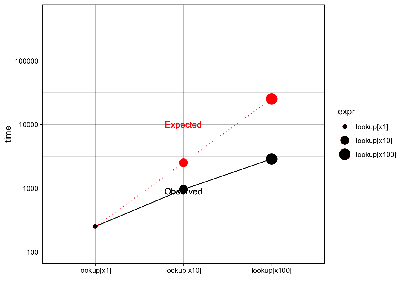
Vectorisation won’t solve every problem, and rather than torturing an existing algorithm into one that uses a vectorised approach, you’re often better off writing your own vectorised function in C++.
Avoid copies
A source of slow R code is growing an object with a loop.
Whenever you use c(), append(),
cbind(), rbind(), or paste() to
create a bigger object, R MUST:
- allocate space for the new object
- copy the old object to its new home.
If you’re repeating this many times, like in a for loop, this can be quite expensive.
Let’s generate some random strings, and then combine them either
iteratively with a loop using collapse(), or in a single
pass using paste().
Note that the performance of collapse() gets relatively
worse as the number of strings grows: combining 100 strings takes almost
30 times longer than combining 10 strings.
random_string <- function() {
  paste(sample(letters, 50, replace = TRUE), collapse = "")
}

strings10 <- replicate(10, random_string())

strings100 <- replicate(100, random_string())

collapse <- function(xs) {
  out <- ""
  for (x in xs) {
    out <- paste0(out, x)
  }
  out
}

# Benchmark

stats = microbenchmark(

  # LOOP *****************
  loop10  = collapse(strings10),
  loop100 = collapse(strings100),

  # VECTORIZED *****************
  vec10   = paste(strings10, collapse = ""),
  vec100  = paste(strings100, collapse = "")
  , unit='us'
)

stats
## Unit: microseconds
## expr min lq mean median uq max neval cld
## loop10 21.043 21.417 21.99106 21.5635 21.8340 38.375 100 a
## loop100 731.501 734.896 768.56598 736.3750 745.0635 3039.709 100 b
## vec10 4.375 4.459 4.63770 4.5420 4.6670 7.292 100 a
## vec100 31.959 32.459 33.33986 32.8135 33.1675 43.876 100 asuppressPackageStartupMessages(library(plyr))
suppressPackageStartupMessages(library(tidyverse))
sum_stats = ddply(stats, .(expr), summarise
, time=median(time, na.rm=T))
sum_stats$group = "loop"
sum_stats$group[grep("vec", sum_stats$expr)] = "vector"
sum_stats$expr = factor(gsub("\\D","",sum_stats$expr), levels = c("10","100"))
options(scipen=6)
ggplot(sum_stats,aes(x=expr, y=time, group=group, col=group))+
geom_point(size=2, fill='white', pch=21)+geom_line()+
theme_linedraw()+ylab("milliseconds")+xlab("")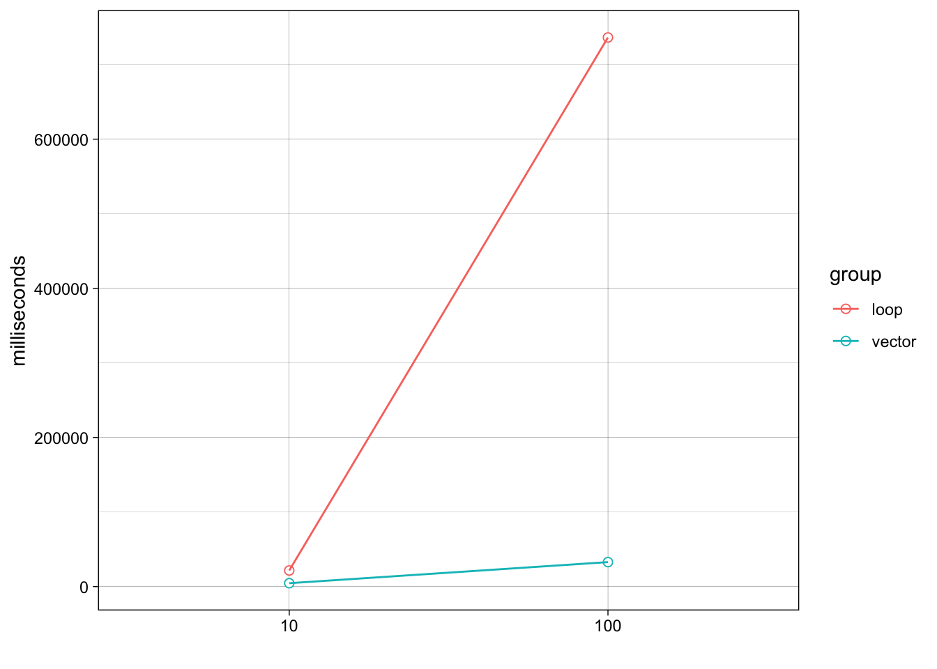
Modifying an object in a loop, e.g., x[i] <- y, can also create a copy, depending on the class of x.
Byte code compilation
R 2.13.0 introduced a byte code compiler which can increase the speed of some code.
A byte code compiler translates a complex high-level language into a very simple language that can be interpreted by a very fast byte code interprete
The following example shows the pure R version of
lapply() from functionals. Compiling it gives a
considerable speedup, although it’s still not quite as fast as the C
version provided by base R.
lapply2 <- function(x, f, ...) {
  out <- vector("list", length(x))
  for (i in seq_along(x)) {
    out[[i]] <- f(x[[i]], ...)
  }
  out
}

lapply2_c <- compiler::cmpfun(lapply2)

x <- list(1:10, letters, c(F, T), NULL)

stats = microbenchmark(
  lapply(x, is.null),
  lapply2(x, is.null),
  lapply2_c(x, is.null),
  unit='us'
)

stats
## Unit: microseconds
## expr min lq mean median uq max neval cld
## lapply(x, is.null) 1.542 1.667 1.95567 1.709 1.7295 24.209 100 a
## lapply2(x, is.null) 1.584 1.668 29.13029 1.709 1.7930 2739.292 100 a
## lapply2_c(x, is.null) 1.625 1.668 1.75392 1.709 1.7930 2.418 100 aByte code compilation really helps here, but in most cases you’re more likely to get a 5-10% improvement.
All base R functions are byte code compiled by default.
Case study: t-test
Imagine we have run 1000 experiments (rows), each of which collects data on 50 individuals (columns).
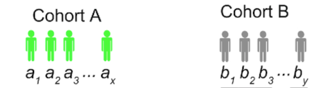
The first 25 individuals in each experiment are assigned to group 1 and the rest to group 2.
We’ll first generate some random data to represent this problem:
m <- 1000 # experiments
n <- 50 # individuals
X <- matrix(rnorm(m * n, mean = 10, sd = 3), nrow = m)
grp <- rep(1:2, each = n / 2)

str(X)
## num [1:1000, 1:50] 10.56 9.57 13.58 4.32 12.28 ...For data in this form, there are two ways to use
t.test(). We can either use the formula interface
or provide two vectors, one for each group.
# for 1,000 exoeriments I run the t.test
# FORMULA
system.time(for(i in 1:m) t.test(X[i, ] ~ grp)$stat)
## user system elapsed
## 0.562 0.011 0.575# VECTORS
system.time(for(i in 1:m) t.test(X[i, grp == 1], X[i, grp == 2])$stat)## user system elapsed
## 0.133 0.001 0.133Timing reveals that the
formula interface is considerably slower.
The for loop computes but doesn’t save the values. We’ll use
apply() to do that. This adds a little overhead:
compT <- function(x, grp){
  t.test(x[grp == 1], x[grp == 2])$stat
}

system.time(t1 <- apply(X, 1, compT, grp = grp))
## user system elapsed
## 0.139 0.002 0.141How can we make this faster?
First, we could try doing less work.
If you look at the source code of
stats:::t.test.default(), you’ll see that it does a lot
more than just compute the t-statistic.
body(stats:::t.test.default)## {
## alternative <- match.arg(alternative)
## if (!missing(mu) && (length(mu) != 1 || is.na(mu)))
## stop("'mu' must be a single number")
## if (!missing(conf.level) && (length(conf.level) != 1 || !is.finite(conf.level) ||
## conf.level < 0 || conf.level > 1))
## stop("'conf.level' must be a single number between 0 and 1")
## if (!is.null(y)) {
## dname <- paste(deparse1(substitute(x)), "and", deparse1(substitute(y)))
## if (paired)
## xok <- yok <- complete.cases(x, y)
## else {
## yok <- !is.na(y)
## xok <- !is.na(x)
## }
## y <- y[yok]
## }
## else {
## dname <- deparse1(substitute(x))
## if (paired)
## stop("'y' is missing for paired test")
## xok <- !is.na(x)
## yok <- NULL
## }
## x <- x[xok]
## if (paired) {
## x <- x - y
## y <- NULL
## }
## nx <- length(x)
## mx <- mean(x)
## vx <- var(x)
## if (is.null(y)) {
## if (nx < 2)
## stop("not enough 'x' observations")
## df <- nx - 1
## stderr <- sqrt(vx/nx)
## if (stderr < 10 * .Machine$double.eps * abs(mx))
## stop("data are essentially constant")
## tstat <- (mx - mu)/stderr
## method <- if (paired)
## "Paired t-test"
## else "One Sample t-test"
## estimate <- setNames(mx, if (paired)
## "mean of the differences"
## else "mean of x")
## }
## else {
## ny <- length(y)
## if (nx < 1 || (!var.equal && nx < 2))
## stop("not enough 'x' observations")
## if (ny < 1 || (!var.equal && ny < 2))
## stop("not enough 'y' observations")
## if (var.equal && nx + ny < 3)
## stop("not enough observations")
## my <- mean(y)
## vy <- var(y)
## method <- paste(if (!var.equal)
## "Welch", "Two Sample t-test")
## estimate <- c(mx, my)
## names(estimate) <- c("mean of x", "mean of y")
## if (var.equal) {
## df <- nx + ny - 2
## v <- 0
## if (nx > 1)
## v <- v + (nx - 1) * vx
## if (ny > 1)
## v <- v + (ny - 1) * vy
## v <- v/df
## stderr <- sqrt(v * (1/nx + 1/ny))
## }
## else {
## stderrx <- sqrt(vx/nx)
## stderry <- sqrt(vy/ny)
## stderr <- sqrt(stderrx^2 + stderry^2)
## df <- stderr^4/(stderrx^4/(nx - 1) + stderry^4/(ny -
## 1))
## }
## if (stderr < 10 * .Machine$double.eps * max(abs(mx),
## abs(my)))
## stop("data are essentially constant")
## tstat <- (mx - my - mu)/stderr
## }
## if (alternative == "less") {
## pval <- pt(tstat, df)
## cint <- c(-Inf, tstat + qt(conf.level, df))
## }
## else if (alternative == "greater") {
## pval <- pt(tstat, df, lower.tail = FALSE)
## cint <- c(tstat - qt(conf.level, df), Inf)
## }
## else {
## pval <- 2 * pt(-abs(tstat), df)
## alpha <- 1 - conf.level
## cint <- qt(1 - alpha/2, df)
## cint <- tstat + c(-cint, cint)
## }
## cint <- mu + cint * stderr
## names(tstat) <- "t"
## names(df) <- "df"
## names(mu) <- if (paired || !is.null(y))
## "difference in means"
## else "mean"
## attr(cint, "conf.level") <- conf.level
## rval <- list(statistic = tstat, parameter = df, p.value = pval,
## conf.int = cint, estimate = estimate, null.value = mu,
## stderr = stderr, alternative = alternative, method = method,
## data.name = dname)
## class(rval) <- "htest"
## rval
## }It also computes the p-value and formats the output for printing.
- We can try to make our code faster by stripping out those pieces.
## my onw function
my_t <- function(x, grp) {

  t_stat <- function(x) {
    m <- mean(x)
    n <- length(x)
    var <- sum( (x - m) ^ 2) / (n - 1)
    list(m = m, n = n, var = var)
  }

  g1 <- t_stat(x[grp == 1])
  g2 <- t_stat(x[grp == 2])
  se_total <- sqrt(g1$var / g1$n + g2$var / g2$n)
  (g1$m - g2$m) / se_total
}

system.time(t2 <- apply(X, 1, my_t, grp = grp))
## user system elapsed
## 0.034 0.000 0.035stopifnot(all.equal(t1, t2))This gives us about a 6x speed improvement.
- Now that we have a fairly simple function, we can make it faster still by vectorising it.
rowtstat <- function(X, grp){

    t_stat <- function(X) {
    m <- rowMeans(X)
    n <- ncol(X)
    var <- rowSums((X - m) ^ 2) / (n - 1)
    list(m = m, n = n, var = var)
  }

  g1 <- t_stat(X[, grp == 1])
  g2 <- t_stat(X[, grp == 2])

  se_total <- sqrt(g1$var / g1$n + g2$var / g2$n)
  (g1$m - g2$m) / se_total
}

system.time(t3 <- rowtstat(X, grp))
## user system elapsed
## 0.016 0.000 0.017stopifnot(all.equal(t1, t3))That’s much faster! It’s at least 40x faster than our previous effort, and around 1000x faster than where we started.
stats = microbenchmark(
   apply(X, 1, my_t, grp = grp)
  ,my_t(X, grp)
  ,rowtstat(X, grp)
  ,unit = "ms"
)

stats
## Unit: milliseconds
## expr min lq mean median uq
## apply(X, 1, my_t, grp = grp) 25.563667 25.951625 26.982882 26.332771 27.118334
## my_t(X, grp) 12.573751 12.656522 12.938545 12.767625 13.047105
## rowtstat(X, grp) 7.680167 7.742084 8.062775 7.871147 7.986605
## max neval cld
## 33.26671 100 c
## 16.90083 100 b
## 13.05454 100 asum_stats = ddply(stats, .(expr), summarise, time=median(time, na.rm=T))
sum_stats$expr = factor(c("T","T_own","Vectorized"), levels = c("T","T_own","Vectorized"))
sum_stats$FC = with(sum_stats, c(1, time[1]/time[2], time[2]/time[3] ))
options(scipen=6)
ggplot(sum_stats,aes(x=expr, y=time))+
geom_line(aes(group=factor(1)),lty='dashed')+
geom_point(aes(fill=expr, size=FC), pch=21, alpha=0.5)+
scale_y_log10(limits = c(1e5,1e8),breaks=c(1e5,1e6,1e7,1e8),labels=c(1e5,1e6,1e7,1e8))+
theme_linedraw()+xlab("")+ylab('milliseconds')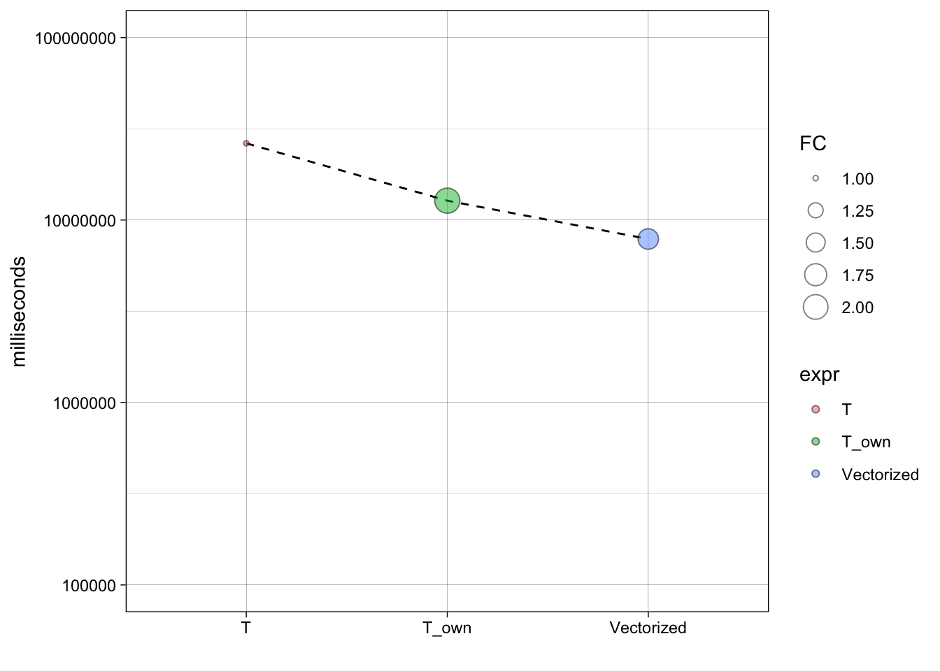
Parallelise
Parallelisation uses multiple cores to work simultaneously on different parts of a problem.
It doesn’t reduce the computing time, but it saves your time because you’re using more of your computer’s resources.
An example of this is lapply() because it operates on
each element independently of the others.
library(parallel)

cores <- detectCores()
cores
## [1] 8pause <- function(i) {
function(x) Sys.sleep(i)
}
system.time(lapply(1:10, pause(0.25)))## user system elapsed
## 0.001 0.001 2.540system.time(mclapply(1:10, pause(0.25), mc.cores = cores))## user system elapsed
## 0.014 0.053 0.525Life is a bit harder in Windows. You need to first
set up a local cluster and then use parLapply():
library(snowfall)

x = list(..of..objects...)


# Initialization
sfInit(parallel=TRUE, cpus=nc, type="SOCK")

#export Functions and data needed by all processes
functionsToCluster <- as.character(lsf.str(envir = .GlobalEnv))
dataToCluster      <- ls()
sfExport(list = c(functionsToCluster, dataToCluster))

#export library needed by all processes
sfLibrary(my_lib)

#set Uniform Random Number Generation
sfClusterSetupRNG()

# run computations
l <- sfLapply(samples, function(x){ .... })

# shut down clusters
sfStop()
There is some communication overhead with parallel computing. If the subproblems are very small, then parallelisation might hurt rather than help. It’s also possible to distribute computation over a network of computers (not just the cores on your local computer) and you can find more information is the high performance computing CRAN task view ( https://cran.r-project.org/web/views/HighPerformanceComputing.html)
A work by Matteo Cereda and Fabio Iannelli