Functions for Vectors and DF

Function	Detail
`range()`	returns a vector containing the min and max of all the given arguments
`summary()`	produces result summaries of data stored in the vector
`unique()`	remove duplicates in the array
`table()`	build a contingency table of the counts at each combination of factor levels
`sort()`	sort a vector
`order()`	order a vector

Transformation of V/DFs

Suppose we want to perform some operations on a dataframe. This can be done using the function with():

d = data.frame(id = 1:6
               , type = c(rep("T",3),rep("U",3)),
                 score = runif(6))


with( d, floor(id/score) )

## [1]  1  5  3 10  6  9

We can make different calculations on a dataframe in one step using transform()

transform(d, useless = floor(id/score) , type = sample(type))

##   id type     score useless
## 1  1    T 0.8658053       1
## 2  2    U 0.3343192       5
## 3  3    U 0.9349960       3
## 4  4    U 0.3882944      10
## 5  5    T 0.7960512       6
## 6  6    T 0.6244655       9

Apply a function

The lapply() and sapply() are useful for working with lists and dataframes. Consider

l = list(   1:5
          , c("a","b")
          , c(T,F,T,T) )

# apply length to the list elements
lapply(l, length)

## [[1]]
## [1] 5
## 
## [[2]]
## [1] 2
## 
## [[3]]
## [1] 4

The function length() is applied to each element of a list and the result is also a list.

Instead, the function sapply() turn the results into a matrix/vector if possible:

sapply(l,length)

## [1] 5 2 4

Functions for DF

Function	Detail
`pairs()`	A quick graphical overview by the scatterplot matrix. Variables are plotted against each other
`xtabs()`	Cross-classifies variables that counts how often a combination of their levels occur
`subset()`	Return subsets of vectors, matrices or data frames which meet conditions

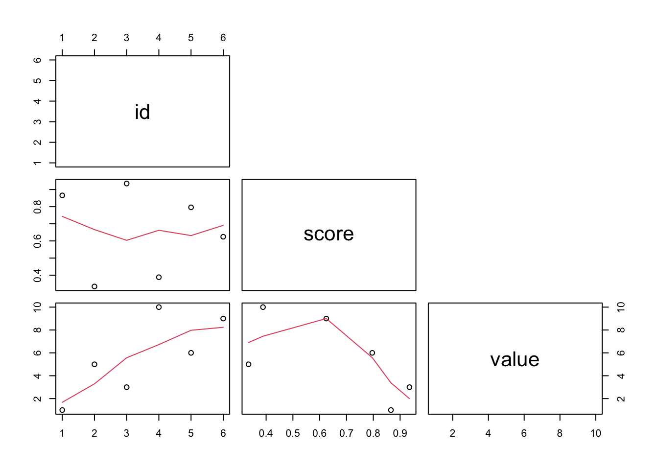
`pairs()`

A quick graphical overview by the scatterplot matrix. Variables are plotted against each other.

The ij-th scatterplot contains x[,i] plotted against x[,j].

d$value=with( d, floor(id/score) )
str(d)

## 'data.frame':    6 obs. of  4 variables:
##  $ id   : int  1 2 3 4 5 6
##  $ type : chr  "T" "T" "T" "U" ...
##  $ score: num  0.866 0.334 0.935 0.388 0.796 ...
##  $ value: num  1 5 3 10 6 9

## quick graphical overview by the scatterplot matrix
pairs(d[,c("id", "score","value")]
      , lower.panel = panel.smooth
      , upper.panel = NULL)

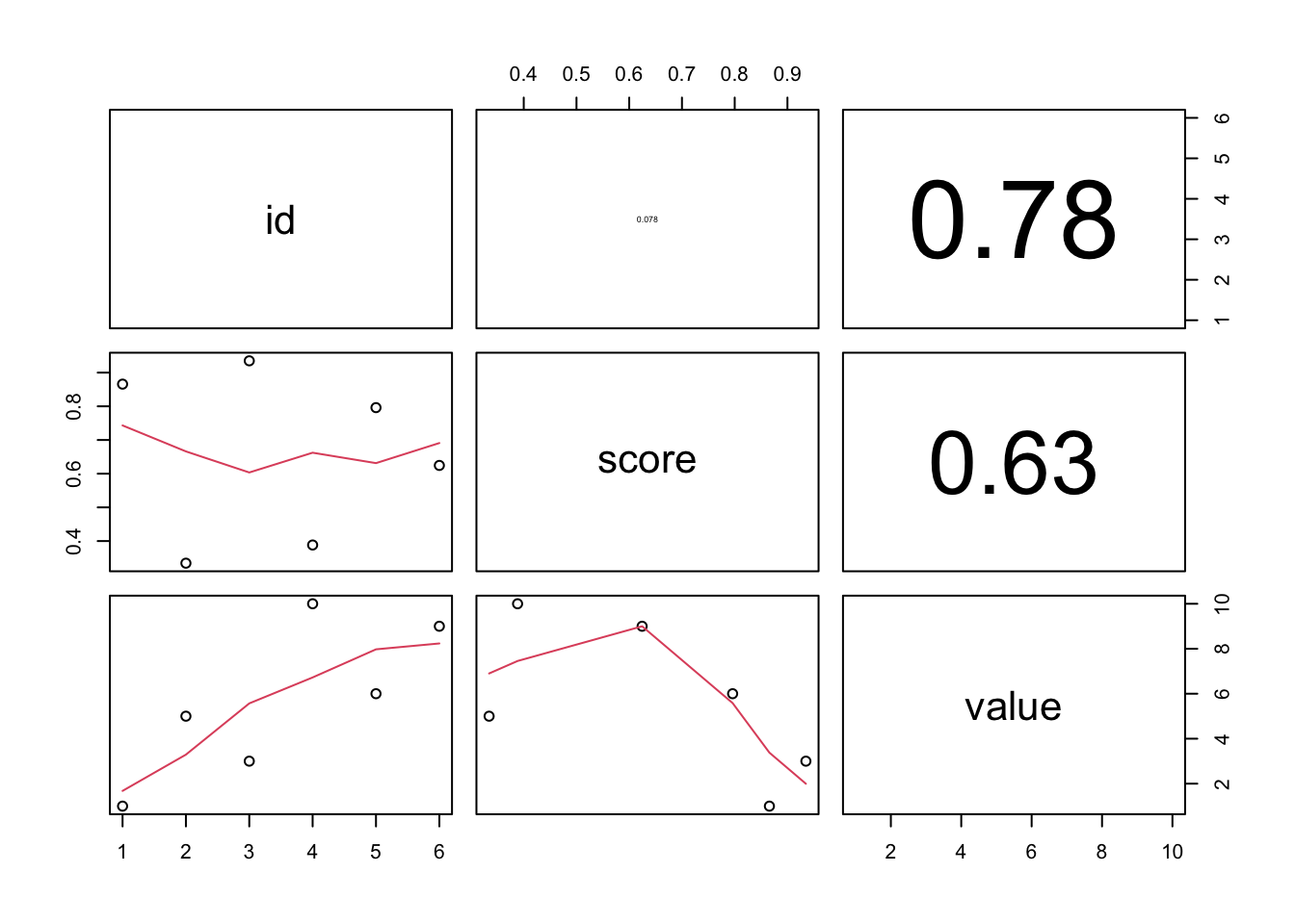
## can make my own panel to show Pearson's Correlation Coefficient (PCC)
panel.cor <- function(x, y, digits = 2, prefix = "", cex.cor, ...){
    usr <- par("usr"); on.exit(par(usr))
    par(usr = c(0, 1, 0, 1))
    r <- abs(cor(x, y))
    txt <- format(c(r, 0.123456789), digits = digits)[1]
    txt <- paste0(prefix, txt)
    if(missing(cex.cor)) cex.cor <- 0.8/strwidth(txt)
    text(0.5, 0.5, txt, cex = cex.cor * r)
}


pairs(d[,c("id", "score","value")]
      , lower.panel = panel.smooth
      , upper.panel = panel.cor) # <-- here!

`xtabs()`

Cross-classifies variables counting how often a combination of their levels occur.

str(d)

## 'data.frame':    6 obs. of  4 variables:
##  $ id   : int  1 2 3 4 5 6
##  $ type : chr  "T" "T" "T" "U" ...
##  $ score: num  0.866 0.334 0.935 0.388 0.796 ...
##  $ value: num  1 5 3 10 6 9

xtabs(~value+type,d)

##      type
## value T U
##    1  1 0
##    3  1 0
##    5  1 0
##    6  0 1
##    9  0 1
##    10 0 1

`subset()`

Return subsets of vectors, matrices or data frames which meet conditions

subset(d, subset = type == "T" & score > 0.5,
          select = c(id, value)
       )

##   id value
## 1  1     1
## 3  3     3

Comparisons

To use filtering effectively, you have to know how to select the observations that you want using the comparison operators.

R provides the standard suite: >, >=, <, <=, != (not equal), and == (equal).

Easy mistakes:

When you’re starting out with R, the easiest mistake to make is to use = instead of == when testing for equality.

subset(d,type = "T")

##   id type     score value
## 1  1    T 0.8658053     1
## 2  2    T 0.3343192     5
## 3  3    T 0.9349960     3
## 4  4    U 0.3882944    10
## 5  5    U 0.7960512     6
## 6  6    U 0.6244655     9

There’s another common problem you might encounter when using ==: floating point numbers. These results might surprise you!
```
sqrt(2) ^ 2 == 2
```
```
## [1] FALSE
```
```
1/49 * 49 == 1
```
```
## [1] FALSE
```
Computers use finite precision arithmetic (they obviously can’t store an infinite number of digits!) so remember that every number you see is an approximation.

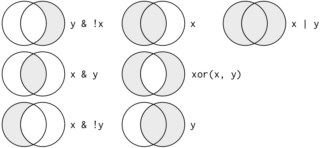
Logical operators

For different types of comparisons/combinations, R provices Boolean operators: & is “and”, | is “or”, and ! is “not”.

Figure shows the complete set of Boolean operations. x is the left-hand circle, y is the right-hand circle, and the shaded region show which parts each operator selects.

A useful short-hand for this problem is x %in% y. This will select every row where x is one of the values in y. We could use it to rewrite the code above:

subset(d, type %in% c("T","F"))

Comparing NAs

One important feature of R that can make comparison tricky are missing values, or NAs (“not availables”).

NA represents an unknown value so missing values are “contagious”: Almost any operation involving an unknown value will also be unknown.

NA > 5

## [1] NA

10 == NA

## [1] NA

NA + 10

## [1] NA

NA / 2

## [1] NA

If you want to determine if a value is missing, use is.na():

is.na(c(1,NA))

## [1] FALSE  TRUE

Functions for Matrices

Function	Detail
`scale()`	To center all columns in a matrix to have mean 0 and to rescale the columns to have variance 1 against each other
`sweep()`	Return an array obtained from an input array by sweeping out a summary statistic

`scale()`

Center all columns in a matrix to have mean=0 and variance=1

If center is TRUE then centering is done by subtracting the column means (omitting NAs) of x from their corresponding columns.

m = matrix(round(runif(9),2),nr=3,nc=3) 
m

##      [,1] [,2] [,3]
## [1,] 0.31 0.31 0.33
## [2,] 0.07 0.43 0.04
## [3,] 0.08 0.42 0.08

#scaling
scale(m, center = TRUE, scale = TRUE)

##            [,1]       [,2]       [,3]
## [1,]  1.1539172 -1.1514402  1.1453126
## [2,] -0.6137858  0.6508140 -0.6999132
## [3,] -0.5401315  0.5006262 -0.4453993
## attr(,"scaled:center")
## [1] 0.1533333 0.3866667 0.1500000
## attr(,"scaled:scale")
## [1] 0.13576941 0.06658328 0.15716234

`sweep()`

Return an array obtained from an input array by sweeping out a summary statistic.

“clean an area thoroughly by brushing away all dirt or litter”

str(m)

##  num [1:3, 1:3] 0.31 0.07 0.08 0.31 0.43 0.42 0.33 0.04 0.08

# median value of each row of the matix
row.med <- apply(m, MARGIN = 1, FUN = median)
row.med

## [1] 0.31 0.07 0.08

# subtracting the median value of each row
sweep(m, MARGIN = 1, STATS = row.med, FUN = "-")

##      [,1] [,2]  [,3]
## [1,]    0 0.00  0.02
## [2,]    0 0.36 -0.03
## [3,]    0 0.34  0.00

A work by Matteo Cereda and Fabio Iannelli

Basic Data Manipulations