Visulizing the costs
Let’s visualize the cost of adding element to an object
We loop through the values 1-N_iter, and save the elapsed time since the beginning for each iteration. The naive way to build our final output is to repeatedly rbind new rows to the end of our dataframe. R is copying the entire dataframe during each iteration. This means that as the dataframe gets bigger, so does the time it takes to copy and allocate the memory. This is the bad way to accumulate data in R.
library(ggplot2)
library(dplyr)
library(ggthemes)

N_iter =1000

finalslow = data.frame(  iteration=0 , time=0)

initialtime = proc.time()[3]

#LOOP + RBIND ********
for(i in 1:N_iter) {
  finalslow = rbind(finalslow, data.frame( iteration = i, time = proc.time()[3]-initialtime))
}

ggplot() +
  geom_line(data=finalslow,aes(x=iteration,y=time),color="red",lwd=1) +
  annotate("text",label="rbind (slowest)",x=N_iter/2,y=max(finalslow$time/3*2),hjust=0.5,color="red",size = 6,angle=15) +
  scale_y_continuous("Time to Complete (seconds)") +
  scale_x_continuous("Loop Iterations") +
  theme_tufte() +
  theme(text=element_text(family="Helvetica"),panel.grid.major.y = element_line(color = "grey95"))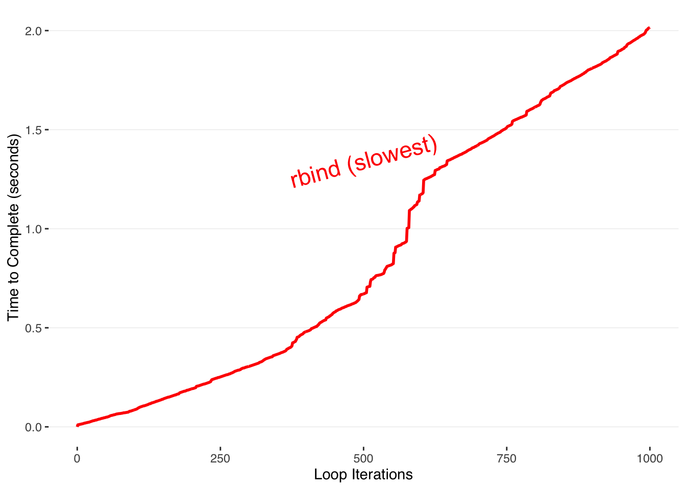
As the number of loops increases, the time required increases quadratically.
This is because at each iteration N of the series, the total number of operations up to that point has been:
\[1+2+3+⋯+N\]
To understand this, we can count the number of operations R is doing under the hood for the entire loop, knowing that each iteration involves R copying the entire existing dataframe to add the one row on the end (black line).
We can compare that to the number of operations that one would expect if you were simply adding a row onto an existing dataframe without copying it (red line).
# PLOTTING functions for quadratic cost (n*(n+1)/2) --------------
generate_rect_coords = function(n) {
  counter = 1
  rects = list()
  for(i in 1:(n*(n+1)/2)) {
      rects[[counter]] = data.frame(xmin=-2,xmax=-1.5,ymin=i-1,ymax=i)
      counter = counter + 1
  }
  return(do.call(rbind,rects))
}

generate_point_coords = function(n) {
  counter = 1
  points = list()
  points[[counter]] = data.frame(x=0,y=0)
  counter = counter + 1
  for(i in 1:n) {
    points[[counter]] = data.frame(x=i,y=i*(i+1)/2)
    counter = counter + 1
  }
  return(do.call(rbind,points))
}

# PLOTTING functions for linear cost n --------------------
generate_rect_coords_linear = function(n) {
  counter = 1
  rects = list()
  for(i in 1:n) {
      rects[[counter]] = data.frame(xmin=-1,xmax=-0.5,ymin=i-1,ymax=i)
      counter = counter + 1
  }
  return(do.call(rbind,rects))
}

generate_point_coords_linear = function(n) {
  counter = 1
  points = list()
  points[[counter]] = data.frame(x=0,y=0)
  counter = counter + 1
  for(i in 1:n) {
    points[[counter]] = data.frame(x=i,y=i)
    counter = counter + 1
  }
  return(do.call(rbind,points))
}

#memory size
size = 16

ggplot() +
  geom_rect(data=generate_rect_coords(size),aes(xmin=xmin,xmax=xmax,ymin=ymin,ymax=ymax),fill="black",color="white",size=0.25) +
  geom_rect(data=generate_rect_coords_linear(size),aes(xmin=xmin,xmax=xmax,ymin=ymin,ymax=ymax),fill="red",color="white",size=0.25) +
  geom_line(data=generate_point_coords_linear(size),aes(x=x,y=y),lwd=0.5,color="red") +
  geom_line(data=generate_point_coords(size),aes(x=x,y=y),lwd=0.5) +
  geom_segment(data=data.frame(x=-1.5,xend=size,y=size*(size+1)/2,yend=size*(size+1)/2),aes(x=x,xend=xend,y=y,yend=yend),alpha=0.5,linetype="dashed",color="black") +
  geom_segment(data=data.frame(x=-0.5,xend=size,y=size,yend=size),aes(x=x,xend=xend,y=y,yend=yend),alpha=0.5,linetype="dashed",color="red") +
  annotate("text", label="O(n^2)",x=18,y=140,parse=TRUE,size=6) +
  annotate("text", label="O(n)",x=18,y=18,parse=TRUE,size=6) +
  scale_x_continuous("Loop Iteration", limits=c(-2,20)) +
  scale_y_continuous("Total Number of Memory Allocations",limits=c(0,150)) +
  theme_tufte() +
  theme(text=element_text(family="Helvetica"),
        panel.grid.major.y = element_line(color = "grey95"))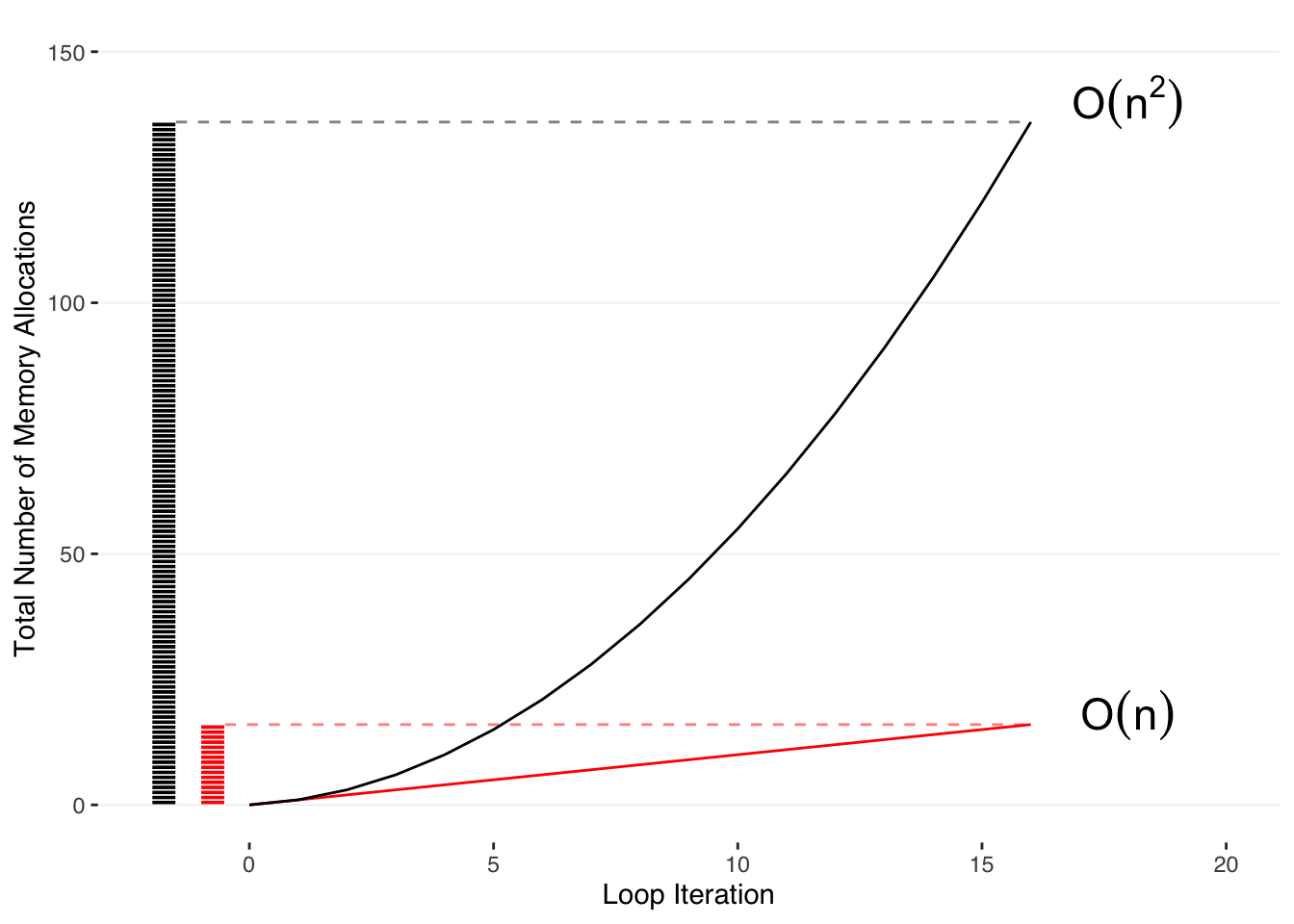
# We can see this is just the series:
\[1+2+3+⋯+N\]
that can also be expressed in terms of the total number of loops, N:
\[\sum_i=N*(N+1)/2\]
So how do you do this correctly?
If you looked at the code above that I used to build the data to plot, you might notice that the functions I wrote to create the data use a list to store the results.
This is because adding an entry to the end of a list does NOT copy the entire data structure during each loop.
Thus, the time it takes to complete scales up linearly with the number of runs. Let’s time how long it takes to accumulate data with this method.
Let’s initialize a list to store our output.
Instead of appending a row to the end of a dataframe on each step, we append only that row to the end of this list.
Unlike the rbind method, this does NOT copy the entire existing dataframe with each iteration.
For a fair comparison, we time the amount of time it takes to both put the list together (the inner loop) as well as combine it into the final dataframe with do.call(). For consistency with the previous method, I call proc.time in the interior loop even though its value isn’t used.
finallist = list()

for(max in 1:N_iter) {
  initialtime = proc.time()[3]
  templist = list()

  # inner loop
  for(i in 1:max) {
    templist[[i]] = data.frame(iteration = i, time = proc.time()[3] - initialtime)
  }
  temp = do.call(rbind,templist)

  finallist[[max]] = data.frame(iteration=max,time = proc.time()[3] - initialtime)
}

# Now we combine all of the dataframe rows in the list into one large dataframe, using the function `do.call()`.

finalfast = do.call(rbind,finallist)
ggplot() +
geom_line(data=finalslow,aes(x=iteration,y=time),color="red",lwd=1) +
geom_line(data=finalfast,aes(x=iteration,y=time),color="blue",lwd=1) +
annotate("text",label="rbind (slowest)",x=N_iter/2,y=max(finalslow$time)/3*2,hjust=0.5,color="red",size = 4,angle=10) +
annotate("text",label="list of rows (faster)",x=N_iter/2,y=max(finalfast$time)/3*2,hjust=1,color="blue",size = 4,angle=10) +
scale_y_continuous("Time to Complete (seconds)") +
scale_x_continuous("Loop Iterations") +
theme_tufte() +
theme(text=element_text(family="Helvetica"),
panel.grid.major.y = element_line(color = "grey90"))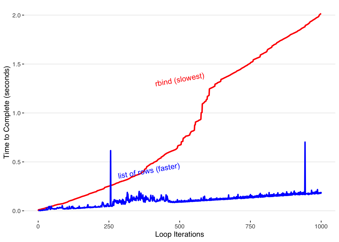
By appending to the end of a list and rbind-ing the whole dataframe together at the end the time it takes to build our completed dataframe only increases linearly with each iteration.
To speed up our loops, we need to know how R operates under the hood. R dataframes aren’t ideal when accumulating data row by row. One of the reasons dataframes are slow is because they perform additional checks every time you add new data.
If speed is really your highest priority, you can forgot the dataframes and accumulate your data in vectors within lists.
Rather than filling each list entry with a row of a dataframe, we can create a list with two entries, each containing a R vector to which we add our data. This is still able to be transformed into a dataframe with do.call() because dataframes are just structured as a collection of lists shown as columns.
faster_final = list()

for(max in 1:N_iter) {
  templist = list(iteration=0, time=0)
  #templist = list() in the previous version
  initialtime = proc.time()[3]

  for(i in 1:max) {
    templist$iteration[i] = i
    templist$time[i] = proc.time()[3] - initialtime
  }
  temp = do.call(rbind,templist)

  faster_final[[max]] = data.frame(iteration=max,time = proc.time()[3] - initialtime)
}

fastest = do.call(rbind,faster_final)

ggplot() +
  geom_line(data=finalslow,aes(x=iteration,y=time),color="red",lwd=1) +
  geom_line(data=finalfast,aes(x=iteration,y=time),color="blue",lwd=1) +
  geom_line(data=fastest,aes(x=iteration,y=time),color="black",lwd=1) +
  annotate("text",label="rbind (slowest)",x=N_iter/2,y=max(finalslow$time)/3*2,hjust=0.5,color="red",size = 4,angle=10) +
  annotate("text",label="list of rows (faster)",x=N_iter/2,y=max(finalfast$time)/3*2,hjust=1,color="blue",size = 4,angle=10) +
   annotate("text",label="list of vectors (even faster)",x=N_iter/3*2.8,y=0.001,hjust=1,color="black",size = 4,angle=0) +
  theme_tufte() +
  scale_y_continuous("Time to Complete (seconds)") +
  scale_x_continuous("Loop Iterations") +
  theme(text=element_text(family="Helvetica"),
        panel.grid.major.y = element_line(color = "grey90"))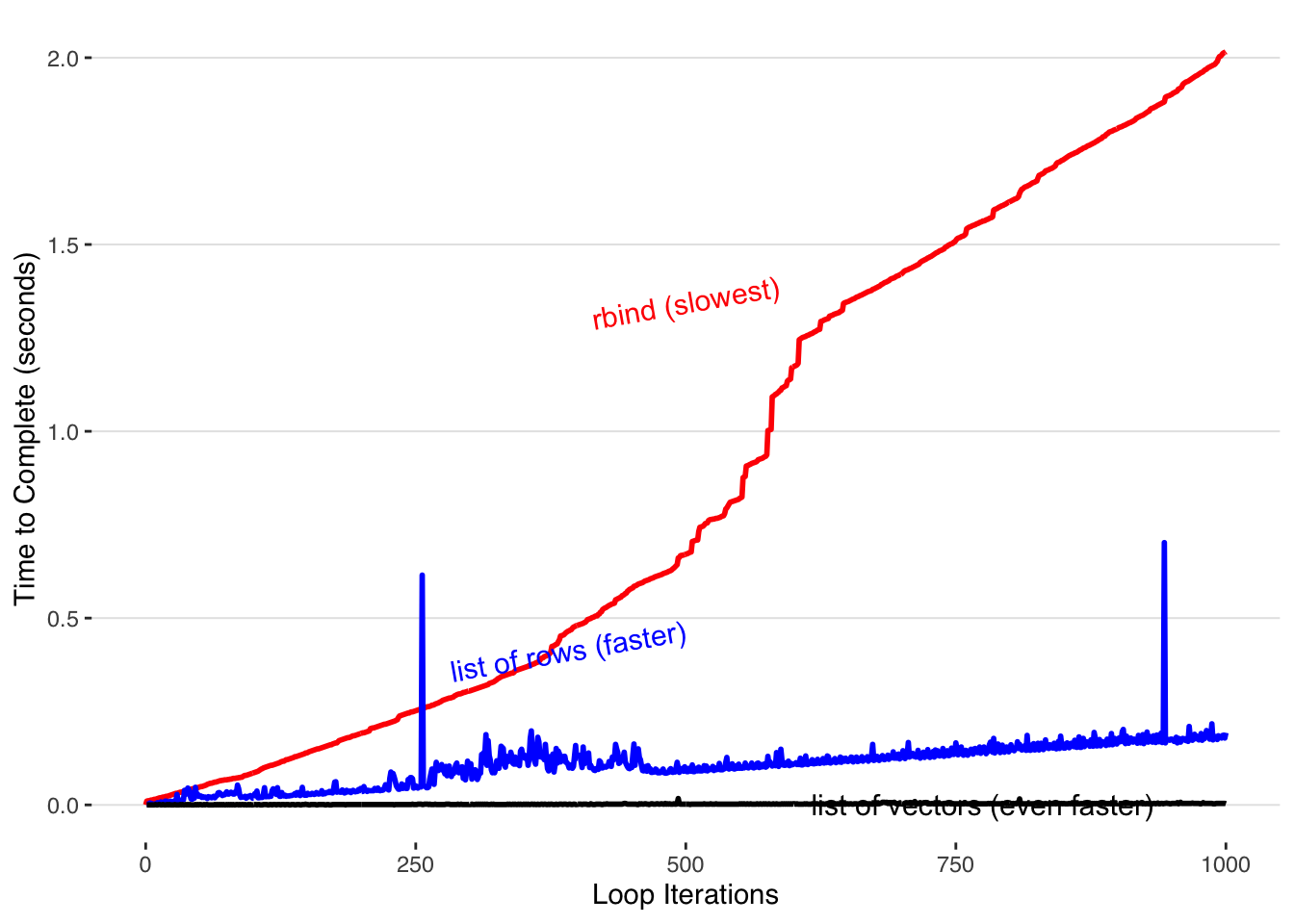
We must go faster. We can do this by pre-allocating our vectors before we accumulate into them.
fastest_final = list()

for(max in 1:N_iter) {

  initialtime = proc.time()[3]
  templist = list()
  #pre-allocating ---------
  templist$iteration = rep(0,N_iter)
  templist$time = rep(0,N_iter)
  #-------------------------

  for(i in 1:max) {
    templist$iteration[i] = i
    templist$time[i] = proc.time()[3] - initialtime
  }

  temp = do.call(rbind,templist)

  fastest_final[[max]] = data.frame(iteration=max,time = proc.time()[3] - initialtime)
}

fastestest = do.call(rbind,fastest_final)

ggplot() +
  geom_line(data=finalslow,aes(x=iteration,y=time),color="red",size=0.5) +
  geom_line(data=finalfast,aes(x=iteration,y=time),color="blue",size=0.5) +
  geom_line(data=fastest,aes(x=iteration,y=time),color="black",size=0.5) +
  geom_line(data=fastestest,aes(x=iteration,y=time),color="darkgreen",size=0.5) +
  annotate("text",label="rbind (slowest)",x=N_iter/2,y=max(finalslow$time)/3*2,hjust=0.5,color="red",size = 4,angle=10) +
  annotate("text",label="list of rows (faster)",x=N_iter/2,y=max(finalfast$time)/3*2,hjust=1,color="blue",size = 4,angle=10) +
  annotate("text",label="list of vectors (even faster)",x=N_iter/3*2.8,y=0.012,hjust=1,color="black",size = 4,angle=0) +
  annotate("text",label="preallocated list of vectors (fastest)",x=N_iter/3*2.8,y=0.008,hjust=1,color="darkgreen",size = 4,angle=0) +
  theme_tufte() + scale_y_log10("Time to Complete (seconds)")+
  # scale_y_continuous() + #limits=c(-0.1,3.3),
  scale_x_continuous("Loop Iterations",expand=c(0,0)) +
  theme(text=element_text(family="Helvetica"),
        panel.grid.major.y = element_line(color = "grey90"))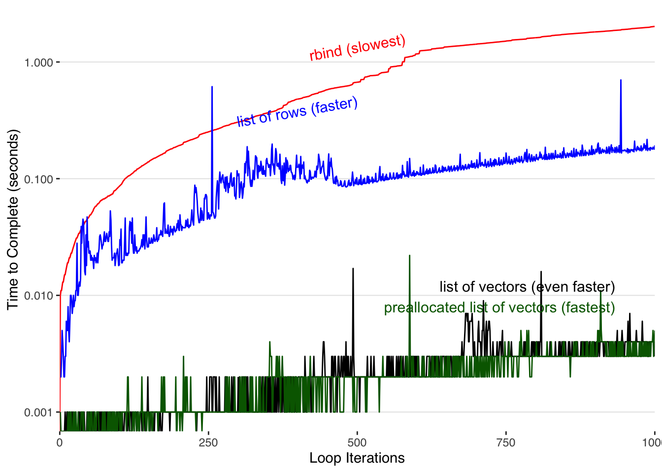
Pre-allocating our vectors within our list results in the best performance.
One downside of pre-allocating memory arises when you’re running a dynamic loop with an unknown duration and you exceed your preallocated memory.
What happens when you overflow this amount? we can simulate the same process as above, except now we have only pre-allocated half of the required memory.
half_allocate = list()

for(max in 1:N_iter) {
  initialtime = proc.time()[3]
  templist = list()

  # Half allocation
  templist$iteration = rep(0,N_iter/2)
  templist$time = rep(0.0,N_iter/2)

  for(i in 1:max) {
    templist$iteration[i] = i
    templist$time[i] = proc.time()[3] - initialtime
  }

  temp = do.call(rbind,templist)

  half_allocate[[max]] = data.frame(iteration=max,time = proc.time()[3] - initialtime)
}

half_allocate_df = do.call(rbind,half_allocate)

fastest$time = fastest$time-.00001
fastestest$time = fastestest$time-.00001
half_allocate_df$time = half_allocate_df$time-.00001

ggplot() +
  geom_point(data=subset(fastestest, iteration<=N_iter/2), aes(x = as.factor(1), y=mean(time)),color="green",size=2) +
  geom_point(data=subset(fastestest, iteration>N_iter/2), aes(x = as.factor(2), y=mean(time)),color="green",size=2) +
  geom_point(data=subset(half_allocate_df, iteration<=N_iter/2), aes(x = as.factor(1), y=mean(time)),color="red",size=2) +
  geom_point(data=subset(half_allocate_df, iteration>N_iter/2), aes(x = as.factor(2), y=mean(time)),color="red",size=2)+
  theme_tufte() +
  scale_y_continuous("Time to Complete (seconds)") +
  theme(text=element_text(family="Helvetica"),
        panel.grid.major.y = element_line(color = "grey90"))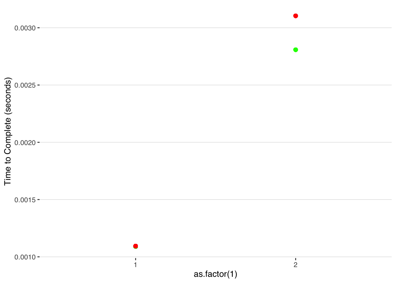
Once we exceed our original preallocated slots, R allocates new memory on the fly and thus the time-to-complete starts increasing from that point at the same rate as in the unallocated case.
A work by Matteo Cereda and Fabio Iannelli