Bioconductor for genomic data
Bioconductor
Bioconductor is an open software development for computational biology and bioinformatics.
It’s open-source because anybody can read and modify the underlying code.
It’s open-development because anybody can contribute and participate in the development of the code.
Analysis and comprehension of high-throughput genomic data
Bioconductor speaks the R language and provides access to powerful statistical and graphical methods for the analysis of genomic data. It also facilitates the integration of biological metadata like GenBank, GO, and PubMed in the analysis of experimental data.
Bioconductor allows the rapid development of extensible, interoperable, and scalable software. Also, high-quality documentation and reproducible research can be promoted using Bioconductor.
Bioconductor website includes materials on how to install, learn, use and contribute back to Bioconductor projects.
Bioconductor goals
To provide access to powerful statistical and graphical methods for the analysis of genomic data.
To facilitate biological metadata integration (e.g.,Gene Ontology, PubMed) in the analysis of experimental data.
To allow the rapid development of extensible, interoperable, and scalable software.
To promote high-quality documentation and reproducible research.
To provide training in computational and statistical methods.
Bioconductor packages
Bioconductor software consists of R add-on packages
An R package is a structured collection of code (R, C++, or other), documentation, and data for performing specific types of analyses
Installing Bioconductor packages
# R versions ≥ 3.6:
if (!requireNamespace("BiocManager", quietly = TRUE))
    install.packages("BiocManager")

BiocManager::install(c(
    "GenomicRanges",
    "Biostrings",
    "BSgenome",
    "BSgenome.Scerevisiae.UCSC.sacCer3",
    "TxDb.Scerevisiae.UCSC.sacCer3.sgdGene",
    "seqLogo"
))


# For older versions of R:
source("http://www.bioconductor.org/biocLite.R")
biocLite(c(
    "GenomicRanges",
    "Biostrings",
    "BSgenome",
    "BSgenome.Scerevisiae.UCSC.sacCer3",
    "TxDb.Scerevisiae.UCSC.sacCer3.sgdGene",
    "seqLogo"))
Load packages
library(GenomicRanges)
library(Biostrings)
library(BSgenome)
Finding documentation
Bioconductor packages usually have documentation in the form of “vignettes”. These are also available on the Bioconductor website: https://www.bioconductor.org/help/
vignette()
vignette(package="Biostrings")
vignette("BiostringsQuickOverview")
browseVignettes()
Motivating Examples
Were are located my “genomic features” of interest (e.g., genes, exons, CpG islands) on the genome (e.g., chromosome, start, end, strand)?
How can I find the overlap of two genomic features (e.g., does a CpG island overlap the gene promoter)?
The IRanges and GenomicRanges packages provide all the infrastructure needed to deal with genomic features and ranges in R
IRanges
The IRanges package is designed to represent sequences, ranges representing indices along those sequences, and data related to those ranges.
A sequence is an ordered and finite collection of elements, such as a vector of integers – not necessarily only for nucleic acid sequences
Consecutive indices can be represented as a range to save memory and computation, for example, instead of saving c(1,2,3,4,5,6,7) just save 1 and 7 – the start and the end indexes –
A basic IRanges instance is the minimal representation of a range (start, end, width)
myiranges <- IRanges(start=c(5,20,25), end=c(10,30,40))

# Accessor functions
start(myiranges)
## [1] 5 20 25end(myiranges)## [1] 10 30 40width(myiranges)## [1] 6 11 16Like all objects from Bioconductor, myiranges is an “S4”
object.
library(pryr)
otype(myiranges)
## [1] "S4"It has a class, which can be obtained with class(). This
determines:
What “slots” (different elements/fields of an S4 class) it has for storing data.
The functions it can be used with (methods).
Data stored in slots is accessible with @ (similar to
$ for lists), but code that uses accessor functions will be
more generic and less liable to break in future.
myiranges@start## [1] 5 20 25myiranges## IRanges object with 3 ranges and 0 metadata columns:
## start end width
## <integer> <integer> <integer>
## [1] 5 10 6
## [2] 20 30 11
## [3] 25 40 16class(myiranges)## [1] "IRanges"
## attr(,"package")
## [1] "IRanges"methods(class="IRanges")## [1] !
## [2] !=
## [3] [
## [4] [[
## [5] [[<-
## [6] [<-
## [7] %in%
## [8] <
## [9] <=
## [10] ==
## [11] >
## [12] >=
## [13] $
## [14] $<-
## [15] aggregate
## [16] anyDuplicated
## [17] anyNA
## [18] append
## [19] as.character
## [20] as.complex
## [21] as.data.frame
## [22] as.env
## [23] as.factor
## [24] as.integer
## [25] as.list
## [26] as.logical
## [27] as.matrix
## [28] as.numeric
## [29] as.raw
## [30] bindROWS
## [31] by
## [32] c
## [33] cbind
## [34] coerce
## [35] coerce<-
## [36] countOverlaps
## [37] coverage
## [38] cvg
## [39] disjoin
## [40] disjointBins
## [41] distance
## [42] distanceToNearest
## [43] do.call
## [44] droplevels
## [45] duplicated
## [46] elementMetadata
## [47] elementMetadata<-
## [48] elementNROWS
## [49] elementType
## [50] end
## [51] end<-
## [52] eval
## [53] expand
## [54] expand.grid
## [55] export
## [56] extractList
## [57] extractROWS
## [58] FactorToClass
## [59] Filter
## [60] findOverlaps
## [61] flank
## [62] follow
## [63] gaps
## [64] getListElement
## [65] head
## [66] ifelse2
## [67] intersect
## [68] is.na
## [69] is.unsorted
## [70] isDisjoint
## [71] isEmpty
## [72] isNormal
## [73] lapply
## [74] length
## [75] lengths
## [76] makeNakedCharacterMatrixForDisplay
## [77] match
## [78] mcols
## [79] mcols<-
## [80] merge
## [81] mergeROWS
## [82] metadata
## [83] metadata<-
## [84] mid
## [85] mstack
## [86] names
## [87] names<-
## [88] nearest
## [89] normalizeSingleBracketReplacementValue
## [90] NSBS
## [91] Ops
## [92] order
## [93] overlapsAny
## [94] overlapsRanges
## [95] parallel_slot_names
## [96] parallelVectorNames
## [97] pcompare
## [98] pcompareRecursively
## [99] pgap
## [100] pintersect
## [101] poverlaps
## [102] precede
## [103] promoters
## [104] psetdiff
## [105] punion
## [106] range
## [107] ranges
## [108] rank
## [109] rbind
## [110] reduce
## [111] Reduce
## [112] reflect
## [113] relist
## [114] rename
## [115] rep
## [116] rep.int
## [117] replaceROWS
## [118] resize
## [119] restrict
## [120] rev
## [121] revElements
## [122] reverse
## [123] sapply
## [124] selfmatch
## [125] seqinfo
## [126] seqinfo<-
## [127] seqlevelsInUse
## [128] setdiff
## [129] setequal
## [130] setListElement
## [131] shift
## [132] shiftApply
## [133] show
## [134] showAsCell
## [135] slidingWindows
## [136] sort
## [137] split
## [138] split<-
## [139] stack
## [140] start
## [141] start<-
## [142] subset
## [143] subsetByOverlaps
## [144] summary
## [145] table
## [146] tail
## [147] tapply
## [148] threebands
## [149] tile
## [150] transform
## [151] union
## [152] unique
## [153] unlist
## [154] unsplit
## [155] update_ranges
## [156] updateObject
## [157] values
## [158] values<-
## [159] whichFirstNotNormal
## [160] width
## [161] width<-
## [162] window
## [163] window<-
## [164] windows
## [165] with
## [166] within
## [167] xtabs
## [168] xtfrm
## [169] zipdown
## see '?methods' for accessing help and source code# IRanges supports many operations
resize(myiranges, 3, fix="start")## IRanges object with 3 ranges and 0 metadata columns:
## start end width
## <integer> <integer> <integer>
## [1] 5 7 3
## [2] 20 22 3
## [3] 25 27 3resize(myiranges, 3, fix="end")## IRanges object with 3 ranges and 0 metadata columns:
## start end width
## <integer> <integer> <integer>
## [1] 8 10 3
## [2] 28 30 3
## [3] 38 40 3Illustrated view of IRanges
illustrate_iranges <- function(obj) {
    for(i in seq_along(obj))
        cat(rep(" ", start(obj)[i]),
            rep("=", width(obj)[i]),
            "\n", sep="")
}
illustrate_iranges( myiranges )
## ======
## ===========
## ================illustrate_iranges( resize(myiranges, 3, fix="start") )## ===
## ===
## ===illustrate_iranges( resize(myiranges, 3, fix="end") )## ===
## ===
## ===illustrate_iranges( flank(myiranges, 2, start=TRUE) )## ==
## ==
## ==illustrate_iranges( flank(myiranges, 2, start=FALSE) )## ==
## ==
## ==illustrate_iranges( range(myiranges) )## ====================================illustrate_iranges( reduce(myiranges) )## ======
## =====================illustrate_iranges( disjoin(myiranges) )## ======
## =====
## ======
## ==========illustrate_iranges( setdiff(range(myiranges), myiranges) )## =========illustrate_iranges( intersect(myiranges[2], myiranges[3]) )## ======illustrate_iranges( union(myiranges[2], myiranges[3]) )## =====================library("ggsci")
mypal = pal_npg("nrc", alpha = 0.7)(9)
plotRanges <-
function(x, xlim = x, main = deparse(substitute(x)),
col = mypal, sep = 0.5, ...)
{
height <- 0.15
if (is(xlim, "Ranges"))
xlim <- c(min(start(xlim)), max(end(xlim)))
bins <- disjointBins(IRanges(start(x), end(x) + 1))
plot.new()
par(mai=c(0.6, 0.2, 0.6, 0.2))
plot.window(xlim, c(0, max(bins)*(height + sep)))
ybottom <- bins * (sep + height) - height
rect(start(x)-0.5, ybottom, end(x)+0.5, ybottom + height, col = col, ...)
title(main, cex.main=1.5, font.main=1)
axis(1)
}
plotRanges( myiranges )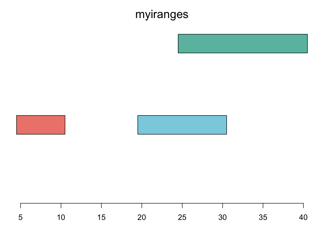
plotRanges( disjoin(myiranges) )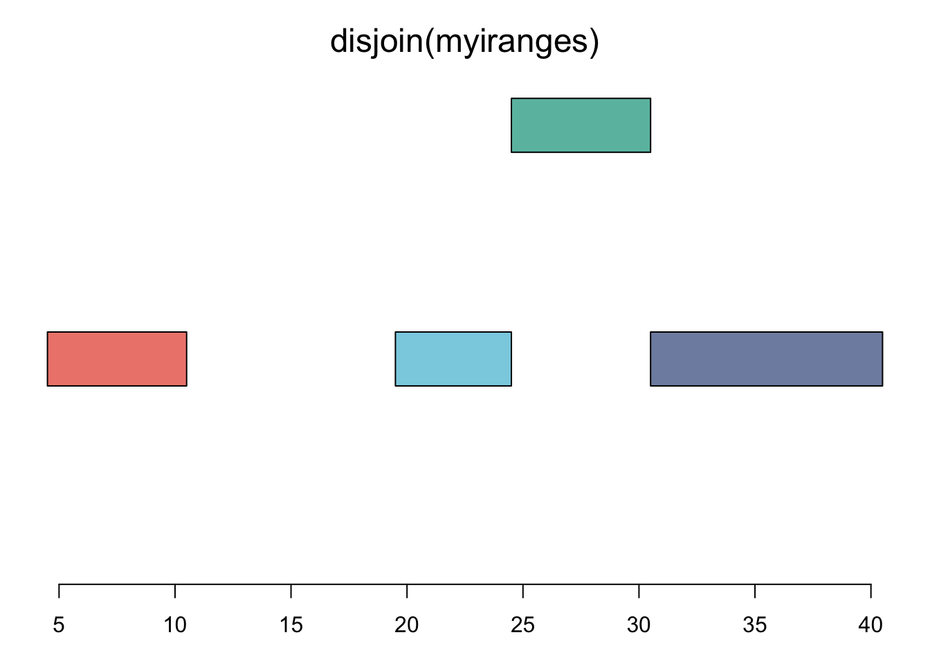
GRanges
Designed to represent genomic intervals (CpG islands, genes, exons, TF binding sites, …)
Based on IRanges package and provides support for other Bioconductor packages (GenomicFeatures, Bsgenome, …)
Contains three major classes:
GRanges: single interval range features – genomic features with single start and end locations
GRangesList: multiple interval range features – features with multiple start/end locations (e.g., a transcript with multiple exons)
GappedAlignments: gapped alignments
To refer to a location in a genome we also need:
- sequence name (chromosome)
- strand, + or -
mygranges <- GRanges(
    seqnames = c("chrII", "chrI", "chrI"),
    ranges = IRanges(start=c(5,20,25), end=c(10,30,40)),
    strand = c("+", "-", "+"))
mygranges
## GRanges object with 3 ranges and 0 metadata columns:
## seqnames ranges strand
## <Rle> <IRanges> <Rle>
## [1] chrII 5-10 +
## [2] chrI 20-30 -
## [3] chrI 25-40 +
## -------
## seqinfo: 2 sequences from an unspecified genome; no seqlengthsclass(mygranges)## [1] "GRanges"
## attr(,"package")
## [1] "GenomicRanges"methods(class="GRanges")## [1] !
## [2] !=
## [3] [
## [4] [[
## [5] [[<-
## [6] [<-
## [7] %in%
## [8] <
## [9] <=
## [10] ==
## [11] >
## [12] >=
## [13] $
## [14] $<-
## [15] aggregate
## [16] anyDuplicated
## [17] anyNA
## [18] append
## [19] as.character
## [20] as.complex
## [21] as.data.frame
## [22] as.env
## [23] as.factor
## [24] as.integer
## [25] as.list
## [26] as.logical
## [27] as.matrix
## [28] as.numeric
## [29] as.raw
## [30] bindROWS
## [31] blocks
## [32] browseGenome
## [33] by
## [34] c
## [35] cbind
## [36] chrom
## [37] chrom<-
## [38] coerce
## [39] countOverlaps
## [40] coverage
## [41] disjoin
## [42] disjointBins
## [43] distance
## [44] distanceToNearest
## [45] do.call
## [46] droplevels
## [47] duplicated
## [48] elementMetadata
## [49] elementMetadata<-
## [50] elementNROWS
## [51] elementType
## [52] end
## [53] end<-
## [54] eval
## [55] expand
## [56] expand.grid
## [57] export
## [58] extractROWS
## [59] FactorToClass
## [60] Filter
## [61] findOverlaps
## [62] flank
## [63] follow
## [64] gaps
## [65] getListElement
## [66] granges
## [67] head
## [68] ifelse2
## [69] intersect
## [70] is.na
## [71] is.unsorted
## [72] isDisjoint
## [73] isEmpty
## [74] lapply
## [75] length
## [76] lengths
## [77] liftOver
## [78] makeNakedCharacterMatrixForDisplay
## [79] match
## [80] mcols
## [81] mcols<-
## [82] merge
## [83] mergeROWS
## [84] metadata
## [85] metadata<-
## [86] mid
## [87] mstack
## [88] names
## [89] names<-
## [90] nearest
## [91] nearestKNeighbors
## [92] normalizeSingleBracketReplacementValue
## [93] Ops
## [94] order
## [95] overlapsAny
## [96] parallel_slot_names
## [97] parallelVectorNames
## [98] pcompare
## [99] pcompareRecursively
## [100] pgap
## [101] pintersect
## [102] poverlaps
## [103] precede
## [104] promoters
## [105] psetdiff
## [106] punion
## [107] range
## [108] ranges
## [109] ranges<-
## [110] rank
## [111] rbind
## [112] reduce
## [113] Reduce
## [114] relist
## [115] relistToClass
## [116] rename
## [117] rep
## [118] rep.int
## [119] replaceROWS
## [120] resize
## [121] restrict
## [122] rev
## [123] revElements
## [124] sapply
## [125] score
## [126] score<-
## [127] selfmatch
## [128] seqinfo
## [129] seqinfo<-
## [130] seqlevelsInUse
## [131] seqnames
## [132] seqnames<-
## [133] setdiff
## [134] setequal
## [135] setListElement
## [136] shift
## [137] shiftApply
## [138] show
## [139] showAsCell
## [140] slidingWindows
## [141] sort
## [142] split
## [143] split<-
## [144] stack
## [145] start
## [146] start<-
## [147] strand
## [148] strand<-
## [149] subset
## [150] subsetByOverlaps
## [151] subtract
## [152] summary
## [153] table
## [154] tail
## [155] tapply
## [156] tile
## [157] transform
## [158] trim
## [159] union
## [160] unique
## [161] unlist
## [162] unsplit
## [163] update_ranges
## [164] update
## [165] updateObject
## [166] values
## [167] values<-
## [168] width
## [169] width<-
## [170] window
## [171] window<-
## [172] windows
## [173] with
## [174] within
## [175] xtabs
## [176] xtfrm
## [177] zipdown
## see '?methods' for accessing help and source code# ?"GRanges-class"
seqnames(mygranges)## factor-Rle of length 3 with 2 runs
## Lengths: 1 2
## Values : chrII chrI
## Levels(2): chrII chrIstrand(mygranges)## factor-Rle of length 3 with 3 runs
## Lengths: 1 1 1
## Values : + - +
## Levels(3): + - *ranges(mygranges)## IRanges object with 3 ranges and 0 metadata columns:
## start end width
## <integer> <integer> <integer>
## [1] 5 10 6
## [2] 20 30 11
## [3] 25 40 16start(mygranges)## [1] 5 20 25end(mygranges)## [1] 10 30 40as.data.frame(mygranges)## seqnames start end width strand
## 1 chrII 5 10 6 +
## 2 chrI 20 30 11 -
## 3 chrI 25 40 16 +# GRanges are like vectors:
mygranges[2]## GRanges object with 1 range and 0 metadata columns:
## seqnames ranges strand
## <Rle> <IRanges> <Rle>
## [1] chrI 20-30 -
## -------
## seqinfo: 2 sequences from an unspecified genome; no seqlengthsmygranges[c(2:3)]## GRanges object with 2 ranges and 0 metadata columns:
## seqnames ranges strand
## <Rle> <IRanges> <Rle>
## [1] chrI 20-30 -
## [2] chrI 25-40 +
## -------
## seqinfo: 2 sequences from an unspecified genome; no seqlengthsc(mygranges, mygranges)## GRanges object with 6 ranges and 0 metadata columns:
## seqnames ranges strand
## <Rle> <IRanges> <Rle>
## [1] chrII 5-10 +
## [2] chrI 20-30 -
## [3] chrI 25-40 +
## [4] chrII 5-10 +
## [5] chrI 20-30 -
## [6] chrI 25-40 +
## -------
## seqinfo: 2 sequences from an unspecified genome; no seqlengths# Like other vectors, elements may be named
names(mygranges) <- c("foo", "fight", "ers")
mygranges## GRanges object with 3 ranges and 0 metadata columns:
## seqnames ranges strand
## <Rle> <IRanges> <Rle>
## foo chrII 5-10 +
## fight chrI 20-30 -
## ers chrI 25-40 +
## -------
## seqinfo: 2 sequences from an unspecified genome; no seqlengths# GRanges can have metadata columns, so they are also a little like data frames:
mygranges$wobble <- c(10, 20, 30)
mygranges## GRanges object with 3 ranges and 1 metadata column:
## seqnames ranges strand | wobble
## <Rle> <IRanges> <Rle> | <numeric>
## foo chrII 5-10 + | 10
## fight chrI 20-30 - | 20
## ers chrI 25-40 + | 30
## -------
## seqinfo: 2 sequences from an unspecified genome; no seqlengths# metadata columns
mcols(mygranges)## DataFrame with 3 rows and 1 column
## wobble
## <numeric>
## foo 10
## fight 20
## ers 30mygranges$wobble## [1] 10 20 30# A handy way to create a GRanges
as("chrI:3-5:+", "GRanges")## GRanges object with 1 range and 0 metadata columns:
## seqnames ranges strand
## <Rle> <IRanges> <Rle>
## [1] chrI 3-5 +
## -------
## seqinfo: 1 sequence from an unspecified genome; no seqlengths# All the operations we saw for IRanges are available for GRanges.
# However most GRanges operations will take strand into account.
#
# Warning: shift() is a notable exception to this.
resize(mygranges, 3, fix="start")## GRanges object with 3 ranges and 1 metadata column:
## seqnames ranges strand | wobble
## <Rle> <IRanges> <Rle> | <numeric>
## foo chrII 5-7 + | 10
## fight chrI 28-30 - | 20
## ers chrI 25-27 + | 30
## -------
## seqinfo: 2 sequences from an unspecified genome; no seqlengthsresize(mygranges, 3, fix="end")## GRanges object with 3 ranges and 1 metadata column:
## seqnames ranges strand | wobble
## <Rle> <IRanges> <Rle> | <numeric>
## foo chrII 8-10 + | 10
## fight chrI 20-22 - | 20
## ers chrI 38-40 + | 30
## -------
## seqinfo: 2 sequences from an unspecified genome; no seqlengthsDNAString and DNAStringSet
DNAString
A DNAString is like a character string of bases “A”, “C”, “G”, “T”, or possibly IUPAC ambiguity codes such as “N” for any base.
myseq <- DNAString("atggaaaccgcgctgctgatttgcgcgtaa")
myseq
## 30-letter DNAString object
## seq: ATGGAAACCGCGCTGCTGATTTGCGCGTAAclass(myseq)## [1] "DNAString"
## attr(,"package")
## [1] "Biostrings"methods(class="DNAString")## [1] !=
## [2] [
## [3] [<-
## [4] %in%
## [5] <
## [6] <=
## [7] ==
## [8] >
## [9] >=
## [10] aggregate
## [11] alphabetFrequency
## [12] anyDuplicated
## [13] anyNA
## [14] append
## [15] as.character
## [16] as.complex
## [17] as.data.frame
## [18] as.env
## [19] as.integer
## [20] as.list
## [21] as.logical
## [22] as.matrix
## [23] as.numeric
## [24] as.raw
## [25] as.vector
## [26] bindROWS
## [27] by
## [28] c
## [29] chartr
## [30] codons
## [31] coerce
## [32] compact
## [33] compareStrings
## [34] complement
## [35] countOverlaps
## [36] countPattern
## [37] countPDict
## [38] countPWM
## [39] duplicated
## [40] elementMetadata
## [41] elementMetadata<-
## [42] eval
## [43] expand
## [44] expand.grid
## [45] extract_character_from_XString_by_positions
## [46] extract_character_from_XString_by_ranges
## [47] extractAt
## [48] extractList
## [49] extractROWS
## [50] FactorToClass
## [51] findOverlaps
## [52] findPalindromes
## [53] hasOnlyBaseLetters
## [54] head
## [55] intersect
## [56] is.na
## [57] isMatchingEndingAt
## [58] isMatchingStartingAt
## [59] lcprefix
## [60] lcsubstr
## [61] lcsuffix
## [62] length
## [63] lengths
## [64] letter
## [65] letterFrequency
## [66] letterFrequencyInSlidingView
## [67] make_XString_from_string
## [68] maskMotif
## [69] masks
## [70] masks<-
## [71] match
## [72] matchLRPatterns
## [73] matchPattern
## [74] matchPDict
## [75] matchProbePair
## [76] matchPWM
## [77] mcols
## [78] mcols<-
## [79] merge
## [80] mergeROWS
## [81] metadata
## [82] metadata<-
## [83] mstack
## [84] nchar
## [85] neditEndingAt
## [86] neditStartingAt
## [87] needwunsQS
## [88] oligonucleotideFrequency
## [89] overlapsAny
## [90] PairwiseAlignments
## [91] PairwiseAlignmentsSingleSubject
## [92] palindromeArmLength
## [93] palindromeLeftArm
## [94] palindromeRightArm
## [95] parallel_slot_names
## [96] pcompare
## [97] pmatchPattern
## [98] rank
## [99] relist
## [100] relistToClass
## [101] rename
## [102] rep
## [103] rep.int
## [104] replaceAt
## [105] replaceLetterAt
## [106] replaceROWS
## [107] rev
## [108] reverse
## [109] reverseComplement
## [110] selfmatch
## [111] seqlevelsInUse
## [112] seqtype
## [113] seqtype<-
## [114] setdiff
## [115] setequal
## [116] shiftApply
## [117] show
## [118] showAsCell
## [119] sort
## [120] split
## [121] split<-
## [122] subseq
## [123] subseq<-
## [124] subset
## [125] subsetByOverlaps
## [126] substr
## [127] substring
## [128] summary
## [129] table
## [130] tail
## [131] tapply
## [132] toComplex
## [133] toString
## [134] transform
## [135] translate
## [136] trimLRPatterns
## [137] twoWayAlphabetFrequency
## [138] union
## [139] unique
## [140] uniqueLetters
## [141] unmasked
## [142] updateObject
## [143] values
## [144] values<-
## [145] vcountPattern
## [146] vcountPDict
## [147] Views
## [148] vmatchPattern
## [149] vmatchPDict
## [150] vwhichPDict
## [151] which.isMatchingEndingAt
## [152] which.isMatchingStartingAt
## [153] whichPDict
## [154] window
## [155] window<-
## [156] with
## [157] xtabs
## [158] xtfrm
## [159] xvcopy
## see '?methods' for accessing help and source code# ?"DNAString-class"
reverseComplement(myseq)## 30-letter DNAString object
## seq: TTACGCGCAAATCAGCAGCGCGGTTTCCATtranslate(myseq)## 10-letter AAString object
## seq: METALLICA*subseq(myseq, 3,5)## 3-letter DNAString object
## seq: GGAalphabetFrequency(myseq)## A C G T M R W S Y K V H D B N - + .
## 7 7 9 7 0 0 0 0 0 0 0 0 0 0 0 0 0 0letterFrequency(myseq, c("AT", "GC"))## A|T G|C
## 14 16# DNAString objects behave like vectors.
myseq[3:5]## 3-letter DNAString object
## seq: GGAc(myseq, myseq)## 60-letter DNAString object
## seq: ATGGAAACCGCGCTGCTGATTTGCGCGTAAATGGAAACCGCGCTGCTGATTTGCGCGTAA# as() converts between types.
as(myseq, "character")## [1] "ATGGAAACCGCGCTGCTGATTTGCGCGTAA"as("ACGT", "DNAString")## 4-letter DNAString object
## seq: ACGTFinding or counting patterns
matchPattern("ATG", myseq)## Views on a 30-letter DNAString subject
## subject: ATGGAAACCGCGCTGCTGATTTGCGCGTAA
## views:
## start end width
## [1] 1 3 3 [ATG]countPattern("ATG", myseq)## [1] 1These functions have arguments to allow for some number of substitutions, or even substitutions, insertions, and deletions.
Use pairwiseAlignment() for more flexible local or
global alignment.
Use matchPWM() for a motif represented as a Position
Weight Matrix.
DNAStringSet
We often want to work with a collection of DNA sequences.
myset <- DNAStringSet(list(chrI=myseq, chrII=DNAString("ACGTACGTAA")))
myset
## DNAStringSet object of length 2:
## width seq names
## [1] 30 ATGGAAACCGCGCTGCTGATTTGCGCGTAA chrI
## [2] 10 ACGTACGTAA chrIIclass(myset)## [1] "DNAStringSet"
## attr(,"package")
## [1] "Biostrings"# ?"DNAStringSet-class"
elementNROWS(myset)## [1] 30 10seqinfo(myset)## Seqinfo object with 2 sequences from an unspecified genome:
## seqnames seqlengths isCircular genome
## chrI 30 NA <NA>
## chrII 10 NA <NA># Since a DNAString is like a vector, a DNAStringSet is has to be like a list.
myset$chrII## 10-letter DNAString object
## seq: ACGTACGTAA# or myset[["chrII"]]
# or myset[[2]]
# Getting sequences with GRanges
getSeq(myset, mygranges[2])## DNAStringSet object of length 1:
## width seq names
## [1] 11 TTACGCGCAAA fightgetSeq(myset, as("chrI:1-3:+", "GRanges"))## DNAStringSet object of length 1:
## width seq
## [1] 3 ATGgetSeq(myset, as("chrI:1-3:-", "GRanges"))## DNAStringSet object of length 1:
## width seq
## [1] 3 CAT# Performs reverse complement if strand is "-".BSgenome and TxDb packages
Genomes and genes for many model organisms are available as Bioconductor packages.
- BSgenome. … - Genomes as DNAStringSet-like objects
- TxDB. … - Genes, transcripts, exons, CDS as GRanges
- org. … - Translation of gene names, assignment to GO categories, etc
Further data may be available using AnnotationHub.
We will be using packages for yeast in this part of the workshop.
library(BSgenome.Scerevisiae.UCSC.sacCer3)
# A yeast genome object has been loaded.
# Actual sequence data is only loaded from disk as needed.
genome <- Scerevisiae
class(genome)
## [1] "BSgenome"
## attr(,"package")
## [1] "BSgenome"# ?"BSgenome-class"
seqinfo(genome)## Seqinfo object with 17 sequences (1 circular) from sacCer3 genome:
## seqnames seqlengths isCircular genome
## chrI 230218 FALSE sacCer3
## chrII 813184 FALSE sacCer3
## chrIII 316620 FALSE sacCer3
## chrIV 1531933 FALSE sacCer3
## chrV 576874 FALSE sacCer3
## ... ... ... ...
## chrXIII 924431 FALSE sacCer3
## chrXIV 784333 FALSE sacCer3
## chrXV 1091291 FALSE sacCer3
## chrXVI 948066 FALSE sacCer3
## chrM 85779 TRUE sacCer3genome$chrM## 85779-letter DNAString object
## seq: TTCATAATTAATTTTTTATATATATATTATATTATA...TACAGAAATATGCTTAATTATAATATAATATCCATAmatchPattern("CAGATA", genome$chrM)## Views on a 85779-letter DNAString subject
## subject: TTCATAATTAATTTTTTATATATATATTATATTA...CAGAAATATGCTTAATTATAATATAATATCCATA
## views:
## start end width
## [1] 731 736 6 [CAGATA]
## [2] 15037 15042 6 [CAGATA]
## [3] 17134 17139 6 [CAGATA]
## [4] 18933 18938 6 [CAGATA]
## [5] 19458 19463 6 [CAGATA]
## [6] 20536 20541 6 [CAGATA]
## [7] 39490 39495 6 [CAGATA]
## [8] 40078 40083 6 [CAGATA]
## [9] 52276 52281 6 [CAGATA]
## [10] 58698 58703 6 [CAGATA]library(TxDb.Scerevisiae.UCSC.sacCer3.sgdGene)
# An object referring to a yeast transcriptome database has been loaded.
txdb <- TxDb.Scerevisiae.UCSC.sacCer3.sgdGene
class(txdb)## [1] "TxDb"
## attr(,"package")
## [1] "GenomicFeatures"Genes have transcripts. Transcripts have exons, and CDSs if they are protein coding.
The GRange for a transcript spans all of its exons. The GRange for a gene spans all the exons of all of its transcripts.
For example:
=============================================== gene

========================  transcript1 of gene
=======   ====  ========  exons of transcript1
   ====   ====  ===       CDSs of transcript1

        ======================================= transcript2 of gene
        ======              ======   ========== exons of transcript2
==== ====== === CDSs of transcript2genes(txdb)## GRanges object with 6534 ranges and 1 metadata column:
## seqnames ranges strand | gene_id
## <Rle> <IRanges> <Rle> | <character>
## Q0010 chrM 3952-4415 + | Q0010
## Q0032 chrM 11667-11957 + | Q0032
## Q0055 chrM 13818-26701 + | Q0055
## Q0075 chrM 24156-25255 + | Q0075
## Q0080 chrM 27666-27812 + | Q0080
## ... ... ... ... . ...
## YPR200C chrXVI 939279-939671 - | YPR200C
## YPR201W chrXVI 939922-941136 + | YPR201W
## YPR202W chrXVI 943032-944188 + | YPR202W
## YPR204C-A chrXVI 946856-947338 - | YPR204C-A
## YPR204W chrXVI 944603-947701 + | YPR204W
## -------
## seqinfo: 17 sequences (1 circular) from sacCer3 genometranscriptsBy(txdb, "gene")## GRangesList object of length 6534:
## $Q0010
## GRanges object with 2 ranges and 2 metadata columns:
## seqnames ranges strand | tx_id tx_name
## <Rle> <IRanges> <Rle> | <integer> <character>
## [1] chrM 3952-4338 + | 6665 Q0010
## [2] chrM 4254-4415 + | 6666 Q0017
## -------
## seqinfo: 17 sequences (1 circular) from sacCer3 genome
##
## $Q0032
## GRanges object with 1 range and 2 metadata columns:
## seqnames ranges strand | tx_id tx_name
## <Rle> <IRanges> <Rle> | <integer> <character>
## [1] chrM 11667-11957 + | 6667 Q0032
## -------
## seqinfo: 17 sequences (1 circular) from sacCer3 genome
##
## $Q0055
## GRanges object with 6 ranges and 2 metadata columns:
## seqnames ranges strand | tx_id tx_name
## <Rle> <IRanges> <Rle> | <integer> <character>
## [1] chrM 13818-16322 + | 6668 Q0050
## [2] chrM 13818-18830 + | 6669 Q0055
## [3] chrM 13818-19996 + | 6670 Q0060
## [4] chrM 13818-21935 + | 6671 Q0065
## [5] chrM 13818-23167 + | 6672 Q0070
## [6] chrM 13818-26701 + | 6673 Q0045
## -------
## seqinfo: 17 sequences (1 circular) from sacCer3 genome
##
## ...
## <6531 more elements>exonsBy(txdb, "tx", use.names=TRUE)## GRangesList object of length 6692:
## $YAL069W
## GRanges object with 1 range and 3 metadata columns:
## seqnames ranges strand | exon_id exon_name exon_rank
## <Rle> <IRanges> <Rle> | <integer> <character> <integer>
## [1] chrI 335-649 + | 1 <NA> 1
## -------
## seqinfo: 17 sequences (1 circular) from sacCer3 genome
##
## $`YAL068W-A`
## GRanges object with 1 range and 3 metadata columns:
## seqnames ranges strand | exon_id exon_name exon_rank
## <Rle> <IRanges> <Rle> | <integer> <character> <integer>
## [1] chrI 538-792 + | 2 <NA> 1
## -------
## seqinfo: 17 sequences (1 circular) from sacCer3 genome
##
## $`YAL067W-A`
## GRanges object with 1 range and 3 metadata columns:
## seqnames ranges strand | exon_id exon_name exon_rank
## <Rle> <IRanges> <Rle> | <integer> <character> <integer>
## [1] chrI 2480-2707 + | 3 <NA> 1
## -------
## seqinfo: 17 sequences (1 circular) from sacCer3 genome
##
## ...
## <6689 more elements>cdsBy(txdb, "tx", use.names=TRUE)## GRangesList object of length 6692:
## $YAL069W
## GRanges object with 1 range and 3 metadata columns:
## seqnames ranges strand | cds_id cds_name exon_rank
## <Rle> <IRanges> <Rle> | <integer> <character> <integer>
## [1] chrI 335-649 + | 1 <NA> 1
## -------
## seqinfo: 17 sequences (1 circular) from sacCer3 genome
##
## $`YAL068W-A`
## GRanges object with 1 range and 3 metadata columns:
## seqnames ranges strand | cds_id cds_name exon_rank
## <Rle> <IRanges> <Rle> | <integer> <character> <integer>
## [1] chrI 538-792 + | 2 <NA> 1
## -------
## seqinfo: 17 sequences (1 circular) from sacCer3 genome
##
## $`YAL067W-A`
## GRanges object with 1 range and 3 metadata columns:
## seqnames ranges strand | cds_id cds_name exon_rank
## <Rle> <IRanges> <Rle> | <integer> <character> <integer>
## [1] chrI 2480-2707 + | 3 <NA> 1
## -------
## seqinfo: 17 sequences (1 circular) from sacCer3 genome
##
## ...
## <6689 more elements>Extracting start codons (I)
To illustrate the use of a TxDb, let us try to extract the start codons of yeast. Our first step is to obtain the locations of the coding sequences.
cds_list <- cdsBy(txdb, "tx", use.names=TRUE)
cds_list
## GRangesList object of length 6692:
## $YAL069W
## GRanges object with 1 range and 3 metadata columns:
## seqnames ranges strand | cds_id cds_name exon_rank
## <Rle> <IRanges> <Rle> | <integer> <character> <integer>
## [1] chrI 335-649 + | 1 <NA> 1
## -------
## seqinfo: 17 sequences (1 circular) from sacCer3 genome
##
## $`YAL068W-A`
## GRanges object with 1 range and 3 metadata columns:
## seqnames ranges strand | cds_id cds_name exon_rank
## <Rle> <IRanges> <Rle> | <integer> <character> <integer>
## [1] chrI 538-792 + | 2 <NA> 1
## -------
## seqinfo: 17 sequences (1 circular) from sacCer3 genome
##
## $`YAL067W-A`
## GRanges object with 1 range and 3 metadata columns:
## seqnames ranges strand | cds_id cds_name exon_rank
## <Rle> <IRanges> <Rle> | <integer> <character> <integer>
## [1] chrI 2480-2707 + | 3 <NA> 1
## -------
## seqinfo: 17 sequences (1 circular) from sacCer3 genome
##
## ...
## <6689 more elements>class(cds_list)## [1] "CompressedGRangesList"
## attr(,"package")
## [1] "GenomicRanges"head( elementNROWS(cds_list) )## YAL069W YAL068W-A YAL067W-A YAL066W YAL064W-B YAL064W
## 1 1 1 1 1 1table( elementNROWS(cds_list) )##
## 1 2 3 4 5 6 8
## 6363 312 12 2 1 1 1cds_list[ elementNROWS(cds_list) >= 2 ]## GRangesList object of length 329:
## $YAL030W
## GRanges object with 2 ranges and 3 metadata columns:
## seqnames ranges strand | cds_id cds_name exon_rank
## <Rle> <IRanges> <Rle> | <integer> <character> <integer>
## [1] chrI 87286-87387 + | 26 <NA> 1
## [2] chrI 87501-87752 + | 27 <NA> 2
## -------
## seqinfo: 17 sequences (1 circular) from sacCer3 genome
##
## $YAL003W
## GRanges object with 2 ranges and 3 metadata columns:
## seqnames ranges strand | cds_id cds_name exon_rank
## <Rle> <IRanges> <Rle> | <integer> <character> <integer>
## [1] chrI 142174-142253 + | 40 <NA> 1
## [2] chrI 142620-143160 + | 41 <NA> 2
## -------
## seqinfo: 17 sequences (1 circular) from sacCer3 genome
##
## $YAL001C
## GRanges object with 2 ranges and 3 metadata columns:
## seqnames ranges strand | cds_id cds_name exon_rank
## <Rle> <IRanges> <Rle> | <integer> <character> <integer>
## [1] chrI 151097-151166 - | 107 <NA> 1
## [2] chrI 147594-151006 - | 106 <NA> 2
## -------
## seqinfo: 17 sequences (1 circular) from sacCer3 genome
##
## ...
## <326 more elements>seqinfo(cds_list)## Seqinfo object with 17 sequences (1 circular) from sacCer3 genome:
## seqnames seqlengths isCircular genome
## chrI 230218 <NA> sacCer3
## chrII 813184 <NA> sacCer3
## chrIII 316620 <NA> sacCer3
## chrIV 1531933 <NA> sacCer3
## chrV 576874 <NA> sacCer3
## ... ... ... ...
## chrXIII 924431 <NA> sacCer3
## chrXIV 784333 <NA> sacCer3
## chrXV 1091291 <NA> sacCer3
## chrXVI 948066 <NA> sacCer3
## chrM 85779 TRUE sacCer3genome(cds_list)## chrI chrII chrIII chrIV chrV chrVI chrVII chrVIII
## "sacCer3" "sacCer3" "sacCer3" "sacCer3" "sacCer3" "sacCer3" "sacCer3" "sacCer3"
## chrIX chrX chrXI chrXII chrXIII chrXIV chrXV chrXVI
## "sacCer3" "sacCer3" "sacCer3" "sacCer3" "sacCer3" "sacCer3" "sacCer3" "sacCer3"
## chrM
## "sacCer3"GRanges and GRangesLists extracted from the txdb have associated seqinfo. Bioconductor will give an error if you try to use them with the wrong genome.
# The ...By functions return GRangesList objects.
# To flatten down to a GRanges, use unlist.
unlist(cds_list)
## GRanges object with 7050 ranges and 3 metadata columns:
## seqnames ranges strand | cds_id cds_name exon_rank
## <Rle> <IRanges> <Rle> | <integer> <character> <integer>
## YAL069W chrI 335-649 + | 1 <NA> 1
## YAL068W-A chrI 538-792 + | 2 <NA> 1
## YAL067W-A chrI 2480-2707 + | 3 <NA> 1
## YAL066W chrI 10091-10399 + | 4 <NA> 1
## YAL064W-B chrI 12046-12426 + | 5 <NA> 1
## ... ... ... ... . ... ... ...
## Q0255 chrM 74495-75622 + | 7030 <NA> 1
## Q0255 chrM 75663-75872 + | 7031 <NA> 2
## Q0255 chrM 75904-75984 + | 7032 <NA> 3
## Q0275 chrM 79213-80022 + | 7033 <NA> 1
## Q0297 chrM 85554-85709 + | 7034 <NA> 1
## -------
## seqinfo: 17 sequences (1 circular) from sacCer3 genome# Note that names will not be unique unless each element has length 1.
cds_ranges <- unlist( range(cds_list) )
start_codons <- resize(cds_ranges, 3, fix="start")
start_seqs <- getSeq(genome, start_codons)
table(start_seqs)## start_seqs
## AGC AGT ATA ATG
## 1 3 6 6682Extracting start codons (II)
The above approach to extracting start codons has a potential flaw: an intron may lie within the start codon.
# An alternative way to get start codons.
cds_seqs <- extractTranscriptSeqs(genome, cds_list)
table( subseq(cds_seqs, 1, 3) )
##
## ATA ATG
## 6 6686It actually happens! “AGC” and “AGT” which we saw previously are gone when we handle introns correctly.
cds_list[ start_seqs == "AGC" ]## GRangesList object of length 1:
## $YIL111W
## GRanges object with 2 ranges and 3 metadata columns:
## seqnames ranges strand | cds_id cds_name exon_rank
## <Rle> <IRanges> <Rle> | <integer> <character> <integer>
## [1] chrIX 155222 + | 3200 <NA> 1
## [2] chrIX 155311-155765 + | 3201 <NA> 2
## -------
## seqinfo: 17 sequences (1 circular) from sacCer3 genomecds_list[ start_seqs == "AGT" ]## GRangesList object of length 3:
## $YJL041W
## GRanges object with 2 ranges and 3 metadata columns:
## seqnames ranges strand | cds_id cds_name exon_rank
## <Rle> <IRanges> <Rle> | <integer> <character> <integer>
## [1] chrX 365784 + | 3523 <NA> 1
## [2] chrX 365903-368373 + | 3524 <NA> 2
## -------
## seqinfo: 17 sequences (1 circular) from sacCer3 genome
##
## $YMR242C
## GRanges object with 2 ranges and 3 metadata columns:
## seqnames ranges strand | cds_id cds_name exon_rank
## <Rle> <IRanges> <Rle> | <integer> <character> <integer>
## [1] chrXIII 754220 - | 5309 <NA> 1
## [2] chrXIII 753225-753742 - | 5308 <NA> 2
## -------
## seqinfo: 17 sequences (1 circular) from sacCer3 genome
##
## $YOR312C
## GRanges object with 2 ranges and 3 metadata columns:
## seqnames ranges strand | cds_id cds_name exon_rank
## <Rle> <IRanges> <Rle> | <integer> <character> <integer>
## [1] chrXV 901194 - | 6397 <NA> 1
## [2] chrXV 900250-900767 - | 6396 <NA> 2
## -------
## seqinfo: 17 sequences (1 circular) from sacCer3 genomeCharacterizing a set of features in a genome
A common need in bioinformatics analyses is to characterize a set of features in a genome: transcription start or end sites, protein binding sites, etc. Bioconductor’s core packages make a first pass at characterization fairly simple. You might then proceed to a specialized tool such as a de-novo motif finder.
As an example, let’s look at sequence upstrand of CDS regions.
library(seqLogo)## Loading required package: grid##
## Attaching package: 'grid'## The following object is masked from 'package:Biostrings':
##
## pattern# let's get 10 nucleotides upstream
upstrand_ranges <- flank(cds_ranges, 10, start=TRUE)
upstrand_seq <- getSeq(genome, upstrand_ranges)
upstrand_seq## DNAStringSet object of length 6692:
## width seq names
## [1] 10 ACGCTAACAA YAL069W
## [2] 10 TCACATCATT YAL068W-A
## [3] 10 GAATGTGGGA YAL067W-A
## [4] 10 AAGCACCATC YAL066W
## [5] 10 CGTCGAAACA YAL064W-B
## ... ... ...
## [6688] 10 TTATTTATTA Q0182
## [6689] 10 ATTTATTAAA Q0250
## [6690] 10 AATTTTTGGA Q0255
## [6691] 10 CAATAAATTT Q0275
## [6692] 10 AATAAATAAT Q0297# counts of each nucleotide
letter_counts <- consensusMatrix(upstrand_seq)
letter_counts## [,1] [,2] [,3] [,4] [,5] [,6] [,7] [,8] [,9] [,10]
## A 2487 2449 2558 2622 2355 2326 2871 3855 2661 2944
## C 1184 1247 1232 1154 1125 1402 1323 632 1461 1192
## G 1038 1091 1092 1112 1239 1058 997 1267 963 1103
## T 1983 1905 1810 1804 1973 1906 1501 938 1607 1453
## M 0 0 0 0 0 0 0 0 0 0
## R 0 0 0 0 0 0 0 0 0 0
## W 0 0 0 0 0 0 0 0 0 0
## S 0 0 0 0 0 0 0 0 0 0
## Y 0 0 0 0 0 0 0 0 0 0
## K 0 0 0 0 0 0 0 0 0 0
## V 0 0 0 0 0 0 0 0 0 0
## H 0 0 0 0 0 0 0 0 0 0
## D 0 0 0 0 0 0 0 0 0 0
## B 0 0 0 0 0 0 0 0 0 0
## N 0 0 0 0 0 0 0 0 0 0
## - 0 0 0 0 0 0 0 0 0 0
## + 0 0 0 0 0 0 0 0 0 0
## . 0 0 0 0 0 0 0 0 0 0# create a proportion table
probs <- prop.table(letter_counts[1:4,], 2)
probs## [,1] [,2] [,3] [,4] [,5] [,6] [,7]
## A 0.3716378 0.3659594 0.3822475 0.3918111 0.3519127 0.3475792 0.4290197
## C 0.1769277 0.1863419 0.1841004 0.1724447 0.1681112 0.2095039 0.1976987
## G 0.1551106 0.1630305 0.1631799 0.1661686 0.1851464 0.1580992 0.1489839
## T 0.2963240 0.2846683 0.2704722 0.2695756 0.2948296 0.2848177 0.2242977
## [,8] [,9] [,10]
## A 0.57606097 0.3976390 0.4399283
## C 0.09444112 0.2183204 0.1781231
## G 0.18933054 0.1439032 0.1648237
## T 0.14016736 0.2401375 0.2171249seqLogo(probs, ic.scale=FALSE)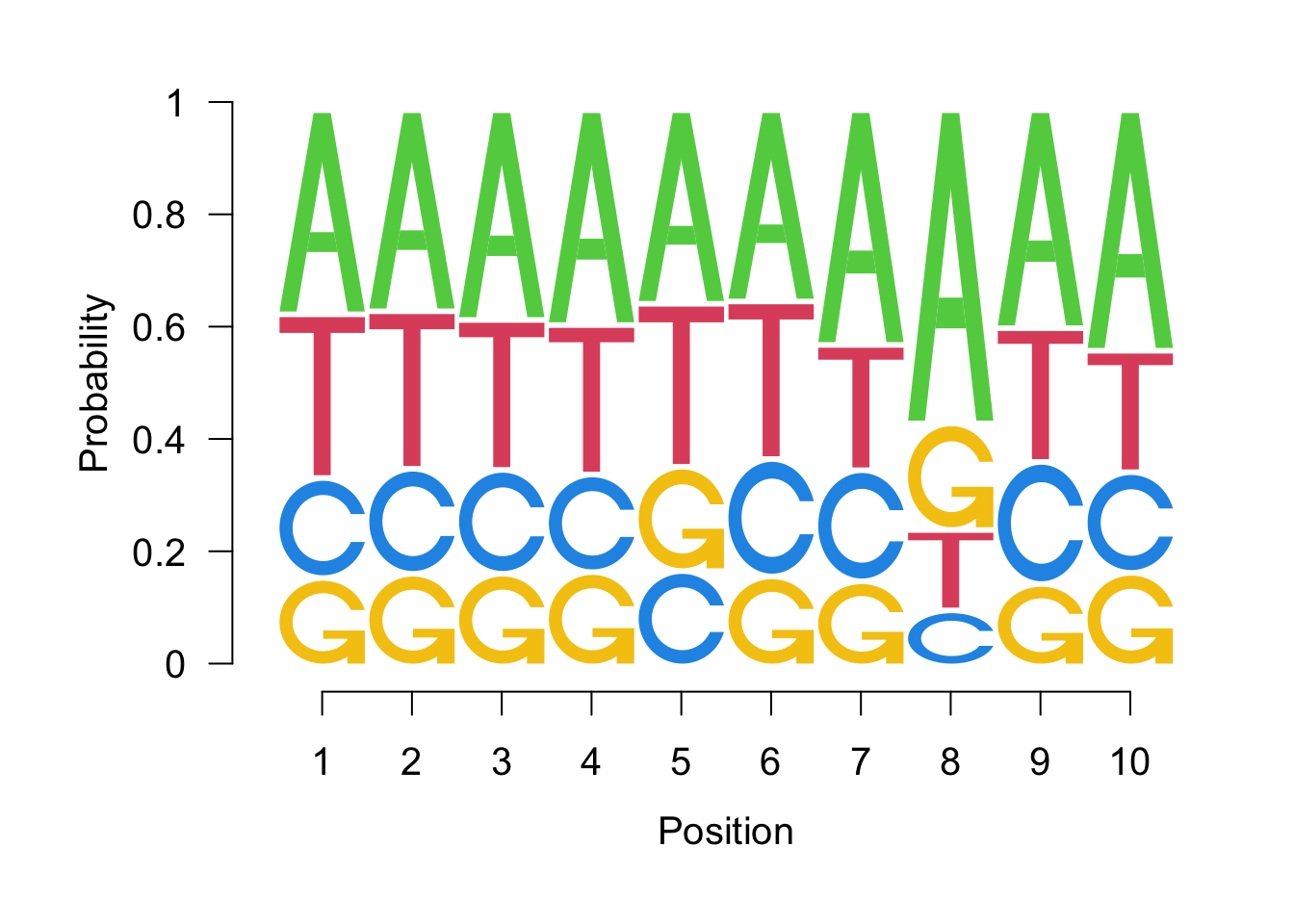
seqLogo(probs)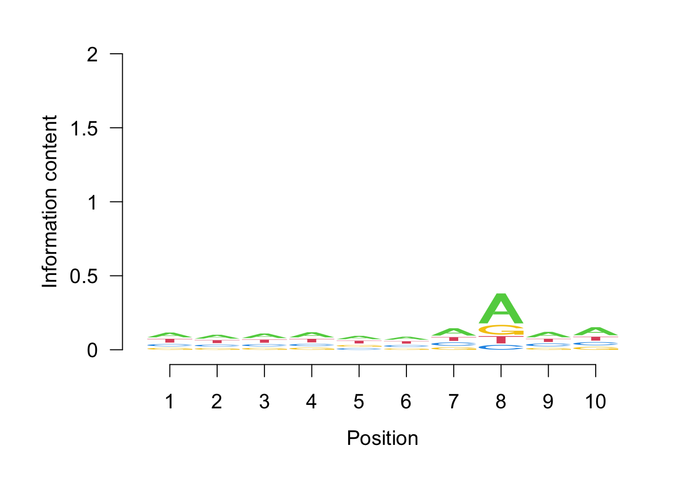
# We may also be interested in k-mer frequencies
colSums( oligonucleotideFrequency(upstrand_seq, 2) )
## AA AC AG AT CA CC CG CT GA GC GG GT TA
## 10308 4067 4450 5359 4993 1703 1610 2454 3653 2079 1657 2468 5687
## TC TG TT
## 2919 2205 4616Annotating detected peaks from a ChIP-seq Analysis
The input for ChIPpeakAnno is a list of called peaks identified from ChIP-seq experiments or any other experiments that yield a set of chromosome coordinates. Although peaks are represented as GRanges in ChIPpeakAnno, other common peak formats such as BED, GFF and MACS can be converted to GRanges easily using a conversion toGRanges method.
The following examples illustrate the usage of this method to convert BED and GFF file to GRanges, add metadata from orignal peaks to the overlap GRanges using function addMetadata, and visualize the overlapping using function makeVennDiagram.
library(ChIPpeakAnno)
bed <- system.file("extdata", "MACS_output.bed", package="ChIPpeakAnno")
gr1 <- toGRanges(bed, format="BED", header=FALSE)
## one can also try import from rtracklayer
gff <- system.file("extdata", "GFF_peaks.gff", package="ChIPpeakAnno")
gr2 <- toGRanges(gff, format="GFF", header=FALSE, skip=3)
## If you are importing files downloaded from ensembl,
## it will be better to import the files into a TxDb object,
## and then convert to GRanges by toGRanges. Here is the sample code:
## library(GenomicFeatures)
## txdb <- makeTxDbFromGFF('/Library/Frameworks/R.framework/Versions/4.2/Resources/library/ChIPpeakAnno/extdata/GFF_peaks.gff')
## anno <- toGRanges(txdb, format='gene')## must keep the class exactly same as gr1$score, i.e., numeric.
gr2$score <- as.numeric(gr2$score)
ol <- findOverlapsOfPeaks(gr1, gr2)## duplicated or NA names found.
## Rename all the names by numbers.## add metadata (mean of score) to the overlapping peaks
ol <- addMetadata(ol, colNames="score", FUN=mean)
ol$peaklist[["gr1///gr2"]][1:2]## GRanges object with 2 ranges and 2 metadata columns:
## seqnames ranges strand | peakNames
## <Rle> <IRanges> <Rle> | <CharacterList>
## [1] chr1 713791-715578 * | gr1__MACS_peak_13,gr2__001,gr2__002
## [2] chr1 724851-727191 * | gr2__003,gr1__MACS_peak_14
## score
## <numeric>
## [1] 850.203
## [2] 29.170
## -------
## seqinfo: 1 sequence from an unspecified genome; no seqlengths# Venn diagram of overlaps for replicated experiments
makeVennDiagram(ol, fill=c("#009E73", "#F0E442"), # circle fill color
col=c("#D55E00", "#0072B2"), #circle border color
cat.col=c("#D55E00", "#0072B2")) # label color, keep same as circle border color## Missing totalTest! totalTest is required for HyperG test.
## If totalTest is missing, pvalue will be calculated by estimating
## the total binding sites of encoding region of human.
## totalTest = humanGenomeSize * (2%(codingDNA) +
## 1%(regulationRegion)) / ( 2 * averagePeakWidth )
## = 3.3e+9 * 0.03 / ( 2 * averagePeakWidth)
## = 5e+7 /averagePeakWidth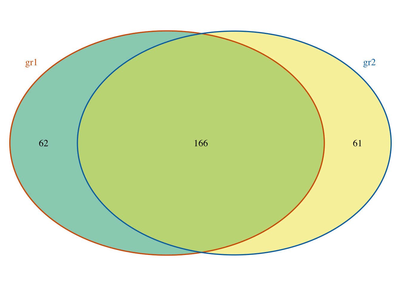
## $p.value
##      gr1 gr2 pval
## [1,]   1   1    0
##
## $vennCounts
##      gr1 gr2 Counts count.gr1 count.gr2
## [1,]   0   0      0         0         0
## [2,]   0   1     61         0        61
## [3,]   1   0     62        62         0
## [4,]   1   1    166       168       169
## attr(,"class")
## [1] "VennCounts"
Prepare annotation data
Annotation data should be an object of GRanges. Same as import peaks, we use the method toGRanges, which can return an object of GRanges, to represent the annotation data. An annotation data be constructed from not only BED, GFF or user defined readable text files, but also EnsDb or TxDb object, by calling the toGRanges method.
library(EnsDb.Hsapiens.v75) ##(hg19)## Loading required package: ensembldb## Loading required package: AnnotationFilter##
## Attaching package: 'ensembldb'## The following object is masked from 'package:stats':
##
## filter## create annotation file from EnsDb or TxDb
annoData <- toGRanges(EnsDb.Hsapiens.v75, feature="gene")## Warning in (function (seqlevels, genome, new_style) : cannot switch some
## GRCh37's seqlevels from NCBI to UCSC styleannoData[1:2]## GRanges object with 2 ranges and 1 metadata column:
## seqnames ranges strand | gene_name
## <Rle> <IRanges> <Rle> | <character>
## ENSG00000223972 chr1 11869-14412 + | DDX11L1
## ENSG00000227232 chr1 14363-29806 - | WASH7P
## -------
## seqinfo: 273 sequences (1 circular) from 2 genomes (hg19, GRCh37)Visualize binding site distribution relative to features
After finding the overlapping peaks, the distribution of the distance of overlapped peaks to the nearest feature such as the transcription start sites (TSS) can be plotted by binOverFeature function. The sample code here plots the distribution of peaks around the TSS.
overlaps <- ol$peaklist[["gr1///gr2"]]
binOverFeature(overlaps, annotationData=annoData,
               radius=5000, nbins=20, FUN=length, errFun=0,
               xlab="distance from TSS (bp)", ylab="count",
               main="Distribution of aggregated peak numbers around TSS")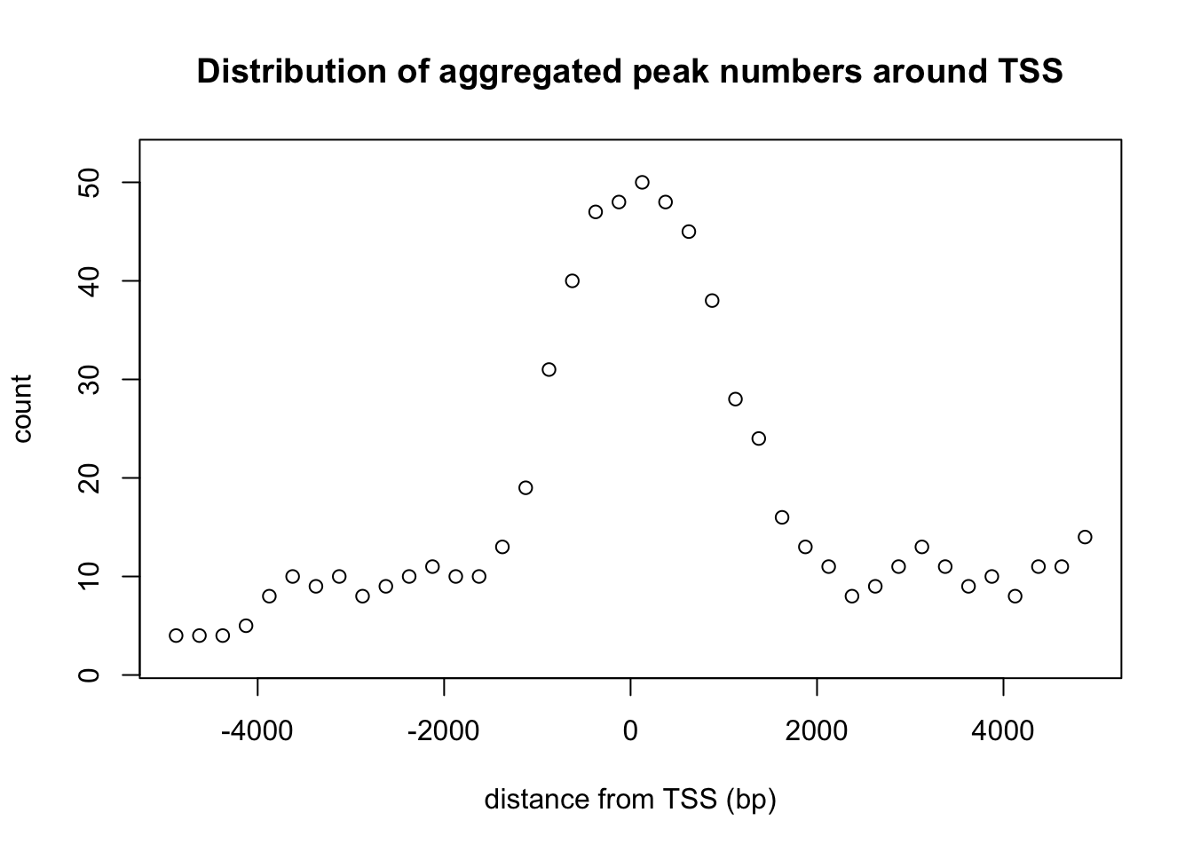
Distribution of peaks around transcript start sites.
In addition, genomicElementDistribution can be used to summarize the distribution of peaks over different type of features such as exon, intron, enhancer, proximal promoter, 5’ UTR and 3’ UTR. This distribution can be summarized in peak centric or nucleotide centric view using the function genomicElementDistribution. Please note that one peak might span multiple type of features, leading to the number of annotated features greater than the total number of input peaks. At the peak centric view, precedence will dictate the annotation order when peaks span multiple type of features.
## check the genomic element distribution of the duplicates
## the genomic element distribution will indicates the
## the correlation between duplicates.
library(TxDb.Hsapiens.UCSC.hg19.knownGene)
peaks <- GRangesList(rep1=gr1,
                     rep2=gr2)
genomicElementDistribution(peaks,
                           TxDb = TxDb.Hsapiens.UCSC.hg19.knownGene,
                           promoterRegion=c(upstream=2000, downstream=500),
                           geneDownstream=c(upstream=0, downstream=2000))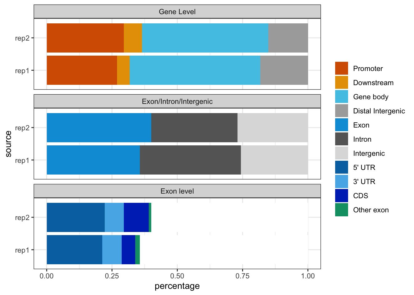
Peak distribution over different genomic features.
## check the genomic element distribution for the overlaps
## the genomic element distribution will indicates the
## the best methods for annotation.
## The percentages in the legend show the percentage of peaks in
## each category.
out <- genomicElementDistribution(overlaps,
                           TxDb = TxDb.Hsapiens.UCSC.hg19.knownGene,
                           promoterRegion=c(upstream=2000, downstream=500),
                           geneDownstream=c(upstream=0, downstream=2000),
                           promoterLevel=list(
                         # from 5' -> 3', fixed precedence 3' -> 5'
                             breaks = c(-2000, -1000, -500, 0, 500),
                             labels = c("upstream 1-2Kb", "upstream 0.5-1Kb",
                                        "upstream <500b", "TSS - 500b"),
                             colors = c("#FFE5CC", "#FFCA99",
                                        "#FFAD65", "#FF8E32")))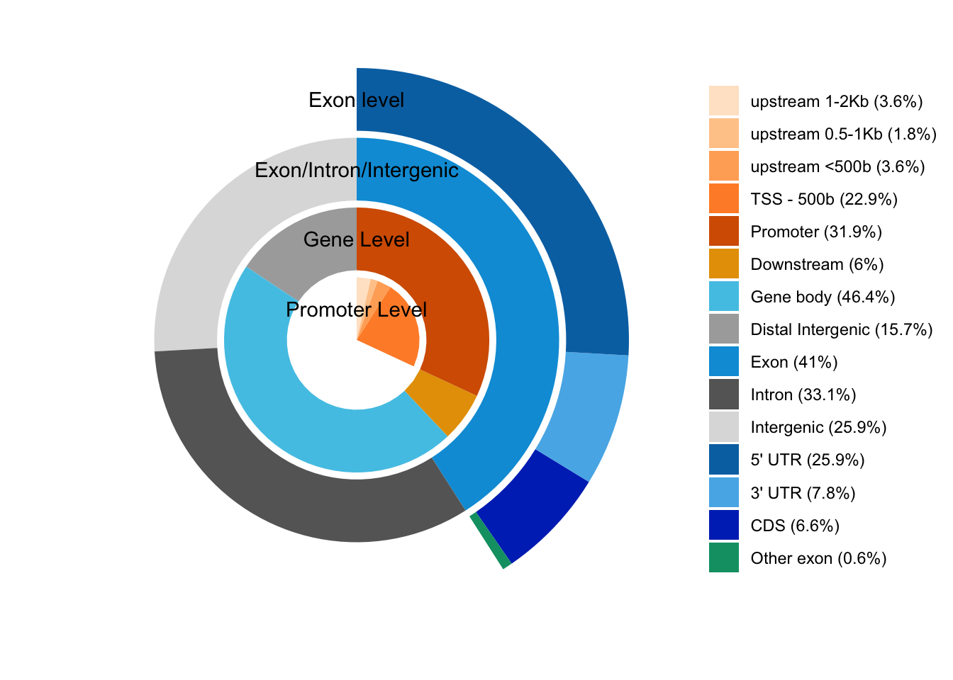
Peak distribution over different genomic features.
## check the genomic element distribution by upset plot.
## by function genomicElementUpSetR, no precedence will be considered.
library(UpSetR)
x <- genomicElementUpSetR(overlaps,
                          TxDb.Hsapiens.UCSC.hg19.knownGene)
## 403 genes were dropped because they have exons located on both strands
## of the same reference sequence or on more than one reference sequence,
## so cannot be represented by a single genomic range.
## Use 'single.strand.genes.only=FALSE' to get all the genes in a
## GRangesList object, or use suppressMessages() to suppress this message.upset(x$plotData, nsets=13, nintersects=NA)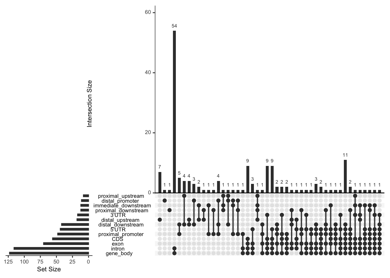
Annotate peaks
As shown from the distribution of aggregated peak numbers around TSS and the distribution of peaks in different of chromosome regions, most of the peaks locate around TSS. Therefore, it is reasonable to use annotatePeakInBatch or annoPeaks to annotate the peaks to the promoter regions of Hg19 genes. Promoters can be specified with bindingRegion. For the following example, promoter region is defined as upstream 2000 and downstream 500 from TSS (bindingRegion=c(-2000, 500)).
overlaps.anno <- annotatePeakInBatch(overlaps,
                                     AnnotationData=annoData,
                                     output="nearestBiDirectionalPromoters",
                                     bindingRegion=c(-2000, 500))
## Annotate peaks by annoPeaks, see ?annoPeaks for details.## maxgap will be ignored.library(org.Hs.eg.db)## overlaps.anno <- addGeneIDs(overlaps.anno,
"org.Hs.eg.db",
IDs2Add = "entrez_id")
head(overlaps.anno)## GRanges object with 6 ranges and 11 metadata columns:
## seqnames ranges strand | peakNames
## <Rle> <IRanges> <Rle> | <CharacterList>
## X1 chr1 713791-715578 * | gr1__MACS_peak_13,gr2__001,gr2__002
## X1 chr1 713791-715578 * | gr1__MACS_peak_13,gr2__001,gr2__002
## X3 chr1 839467-840090 * | gr1__MACS_peak_16,gr2__004
## X4 chr1 856361-856999 * | gr1__MACS_peak_17,gr2__005
## X5 chr1 859315-860144 * | gr2__006,gr1__MACS_peak_18
## X10 chr1 901118-902861 * | gr2__012,gr1__MACS_peak_23
## score peak feature feature.ranges feature.strand
## <numeric> <character> <character> <IRanges> <Rle>
## X1 850.203 X1 ENSG00000228327 700237-714006 -
## X1 850.203 X1 ENSG00000237491 714150-745440 +
## X3 73.120 X3 ENSG00000272438 840214-851356 +
## X4 54.690 X4 ENSG00000223764 852245-856396 -
## X5 81.485 X5 ENSG00000187634 860260-879955 +
## X10 119.910 X10 ENSG00000187583 901877-911245 +
## distance insideFeature distanceToSite gene_name entrez_id
## <integer> <character> <integer> <character> <character>
## X1 0 overlapStart 0 RP11-206L10.2 <NA>
## X1 0 overlapStart 0 RP11-206L10.9 105378580
## X3 123 upstream 123 RP11-54O7.16 <NA>
## X4 0 overlapStart 0 RP11-54O7.3 100130417
## X5 115 upstream 115 SAMD11 148398
## X10 0 overlapStart 0 PLEKHN1 84069
## -------
## seqinfo: 1 sequence from an unspecified genome; no seqlengths# Pie chart of the distribution of common peaks around features.
pie1(table(overlaps.anno$insideFeature))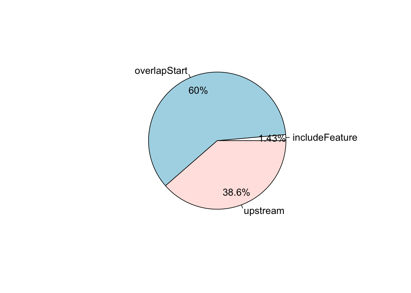
# you can save a csv file with annotated peaks
# write.csv(as.data.frame(unname(overlaps.anno)), "anno.csv")
Obtain enriched GO terms and Pathways
The following example shows how to use getEnrichedGO to obtain a list of enriched GO terms with annotated peaks. For pathway analysis, please use function getEnrichedPATH with reactome or KEGG database. Please note that by default feature_id_type is set as “ensembl_gene_id”. If you are using TxDb as annotation data, please set it to “entrez_id”.
over <- getEnrichedGO(overlaps.anno, orgAnn="org.Hs.eg.db", condense=TRUE)## enrichmentPlot(over)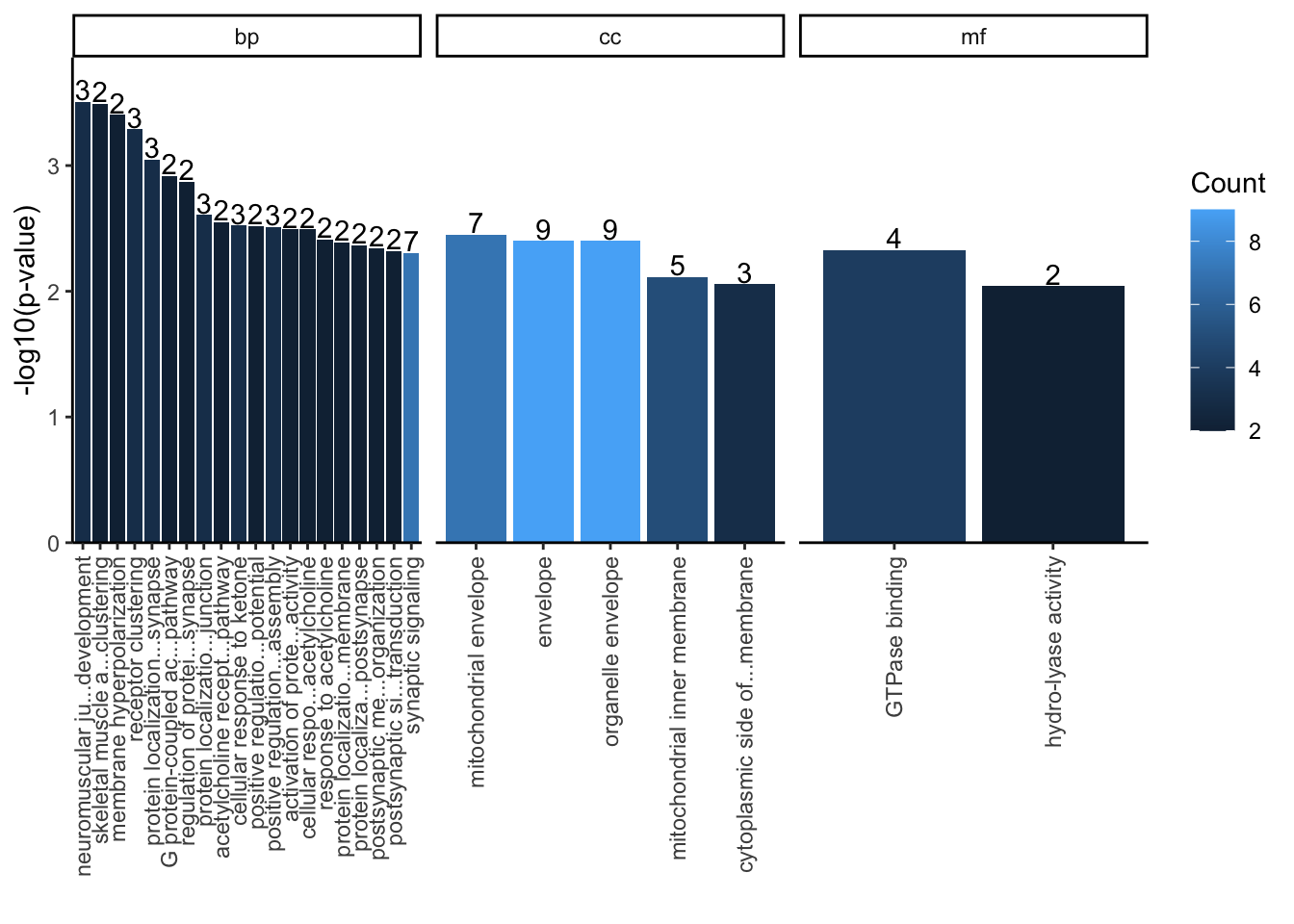
library(reactome.db)
path <- getEnrichedPATH(overlaps.anno, "org.Hs.eg.db", "reactome.db", maxP=.05)
enrichmentPlot(path)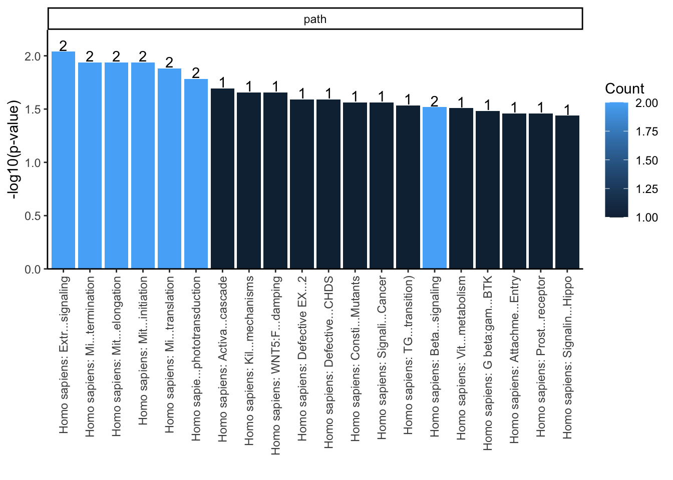
Obtain the sequences surrounding the peaks
Here is an example to get the sequences of the peaks plus 20 bp upstream and downstream for PCR validation or motif discovery.
library(BSgenome.Hsapiens.UCSC.hg19)
seq <- getAllPeakSequence(overlaps, upstream=20, downstream=20, genome=Hsapiens)
# write2FASTA(seq, "peaksequences.fa")
A work by Matteo Cereda and Fabio Iannelli