Relational Data
Introduction
Multiple tables of data are called RELATIONAL DATA .
Relations are always defined between a pair of tables.
There are three families of verbs designed to work with relational data:
| Family | Meaning |
|---|---|
| Mutating joins | add new variables to one data frame from matching observations in another |
| Filtering joins | filter observations from one data frame based on whether or not they match an observation in the other table. |
| Set operations | treat observations as if they were set elements. |
Prerequisites
suppressWarnings(library(tidyverse))
suppressWarnings(library(nycflights13))
nycflights13
We will use the nycflights13 package to learn about relational data.
nycflights13 contains four tibbles that are related to the
flights table that you used in [data transformation]:
airlineslets you look up the full carrier name from its abbreviated code:print(airlines, n=2)## # A tibble: 16 × 2 ## carrier name ## <chr> <chr> ## 1 9E Endeavor Air Inc. ## 2 AA American Airlines Inc. ## # … with 14 more rowsairportsgives information about each airport, identified by thefaaairport code:print(airports, n=2)## # A tibble: 1,458 × 8 ## faa name lat lon alt tz dst tzone ## <chr> <chr> <dbl> <dbl> <dbl> <dbl> <chr> <chr> ## 1 04G Lansdowne Airport 41.1 -80.6 1044 -5 A America/New_York ## 2 06A Moton Field Municipal Airport 32.5 -85.7 264 -6 A America/Chicago ## # … with 1,456 more rowsplanesgives information about each plane, identified by itstailnum:print(planes, n=2)## # A tibble: 3,322 × 9 ## tailnum year type manufacturer model engines seats speed engine ## <chr> <int> <chr> <chr> <chr> <int> <int> <int> <chr> ## 1 N10156 2004 Fixed wing multi engine EMBRAER EMB-14… 2 55 NA Turbo… ## 2 N102UW 1998 Fixed wing multi engine AIRBUS INDUSTRIE A320-2… 2 182 NA Turbo… ## # … with 3,320 more rowsweathergives the weather at each NYC airport for each hour:print(weather, n=2)## # A tibble: 26,115 × 15 ## origin year month day hour temp dewp humid wind_dir wind_speed wind_gust precip ## <chr> <int> <int> <int> <int> <dbl> <dbl> <dbl> <dbl> <dbl> <dbl> <dbl> ## 1 EWR 2013 1 1 1 39.0 26.1 59.4 270 10.4 NA 0 ## 2 EWR 2013 1 1 2 39.0 27.0 61.6 250 8.06 NA 0 ## # … with 26,113 more rows, and 3 more variables: pressure <dbl>, visib <dbl>, ## # time_hour <dttm>
One way to show the relationships between the different tables is with a drawing:
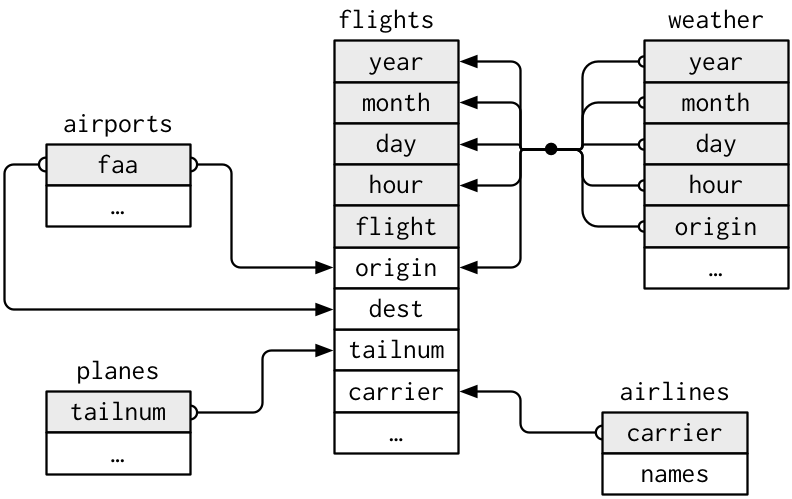
For nycflights13:
flightsconnects toplanesvia a single variable,tailnum.flightsconnects toairlinesthrough thecarriervariable.flightsconnects toairportsin two ways: via theoriginanddestvariables.flightsconnects toweatherviaorigin(the location), andyear,month,dayandhour(the time).
Keys

The variables used to connect each pair of tables are called keys.
A key is a variable (or set of variables) that uniquely identifies an observation.
| Key | Function |
|---|---|
| primary | uniquely identifies an observation in its own table. |
| foreign | uniquely identifies an observation in another table. |
| surrogate | substitute a key |
A variable can be both a primary key and a foreign key.
It’s good practice to verify that they can uniquely identify each observation.
planes %>% count(tailnum) %>% filter(n > 1)## # A tibble: 0 × 2
## # … with 2 variables: tailnum <chr>, n <int>weather %>% count(year, month, day, hour, origin) %>% filter(n > 1)## # A tibble: 3 × 6
## year month day hour origin n
## <int> <int> <int> <int> <chr> <int>
## 1 2013 11 3 1 EWR 2
## 2 2013 11 3 1 JFK 2
## 3 2013 11 3 1 LGA 2Sometimes a table does NOT have an explicit primary key.
Each row is an observation, but no combination of variables reliably identifies it.
For example, what’s the primary key in the flights
table? You might think it would be the date plus the flight or tail
number, but neither of those are unique:
flights %>%
  count(year, month, day, flight) %>%
  filter(n > 1)
## # A tibble: 29,768 × 5
## year month day flight n
## <int> <int> <int> <int> <int>
## 1 2013 1 1 1 2
## 2 2013 1 1 3 2
## 3 2013 1 1 4 2
## 4 2013 1 1 11 3
## 5 2013 1 1 15 2
## 6 2013 1 1 21 2
## 7 2013 1 1 27 4
## 8 2013 1 1 31 2
## 9 2013 1 1 32 2
## 10 2013 1 1 35 2
## # … with 29,758 more rowsflights %>%
count(year, month, day, tailnum) %>%
filter(n > 1)## # A tibble: 64,928 × 5
## year month day tailnum n
## <int> <int> <int> <chr> <int>
## 1 2013 1 1 N0EGMQ 2
## 2 2013 1 1 N11189 2
## 3 2013 1 1 N11536 2
## 4 2013 1 1 N11544 3
## 5 2013 1 1 N11551 2
## 6 2013 1 1 N12540 2
## 7 2013 1 1 N12567 2
## 8 2013 1 1 N13123 2
## 9 2013 1 1 N13538 3
## 10 2013 1 1 N13566 3
## # … with 64,918 more rowsIf a table lacks a primary key, it’s sometimes useful to add one with
mutate()androw_number().
That makes it easier to match observations if you’ve done some filtering and want to check back in with the original data. This is called a surrogate key.

A primary key and the corresponding foreign key in another table form a relation.

Relations are typically one-to-many.
For example, each flight has one plane, but each plane has many flights. In other data, you’ll occasionally see a 1-to-1 relationship. You can think of this as a special case of 1-to-many.
You can model many-to-many relations with a many-to-1 relation plus a 1-to-many relation.
For example, in this data there’s a many-to-many relationship between airlines and airports: each airline flies to many airports; each airport hosts many airlines.
Mutating joins
Like mutate(),
the join functions add variables to the right.
For these examples, we’ll make it easier to see what’s going on in the examples by creating a narrower dataset:
flights2 <- flights %>%
  select(year:day, hour, origin, dest, tailnum, carrier)
flights2
## # A tibble: 336,776 × 8
## year month day hour origin dest tailnum carrier
## <int> <int> <int> <dbl> <chr> <chr> <chr> <chr>
## 1 2013 1 1 5 EWR IAH N14228 UA
## 2 2013 1 1 5 LGA IAH N24211 UA
## 3 2013 1 1 5 JFK MIA N619AA AA
## 4 2013 1 1 5 JFK BQN N804JB B6
## 5 2013 1 1 6 LGA ATL N668DN DL
## 6 2013 1 1 5 EWR ORD N39463 UA
## 7 2013 1 1 6 EWR FLL N516JB B6
## 8 2013 1 1 6 LGA IAD N829AS EV
## 9 2013 1 1 6 JFK MCO N593JB B6
## 10 2013 1 1 6 LGA ORD N3ALAA AA
## # … with 336,766 more rowsImagine you want to add the full airline name to the
flights2 data. You can combine the airlines
and flights2 data frames with left_join():
flights2 %>%
  select(-origin, -dest) %>%
  left_join(airlines, by = "carrier")
## # A tibble: 336,776 × 7
## year month day hour tailnum carrier name
## <int> <int> <int> <dbl> <chr> <chr> <chr>
## 1 2013 1 1 5 N14228 UA United Air Lines Inc.
## 2 2013 1 1 5 N24211 UA United Air Lines Inc.
## 3 2013 1 1 5 N619AA AA American Airlines Inc.
## 4 2013 1 1 5 N804JB B6 JetBlue Airways
## 5 2013 1 1 6 N668DN DL Delta Air Lines Inc.
## 6 2013 1 1 5 N39463 UA United Air Lines Inc.
## 7 2013 1 1 6 N516JB B6 JetBlue Airways
## 8 2013 1 1 6 N829AS EV ExpressJet Airlines Inc.
## 9 2013 1 1 6 N593JB B6 JetBlue Airways
## 10 2013 1 1 6 N3ALAA AA American Airlines Inc.
## # … with 336,766 more rowsUnderstanding joins
To help you learn how joins work, I’m going to use a visual representation:
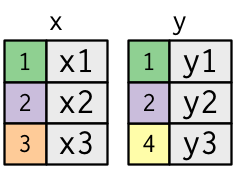
x <- tribble(
  ~key, ~val_x,
     1, "x1",
     2, "x2",
     3, "x3"
)
y <- tribble(
  ~key, ~val_y,
     1, "y1",
     2, "y2",
     4, "y3"
)
The coloured column represents the “key” variable: these are used to match the rows between the tables.
The grey column represents the “value” column that is carried along for the ride.
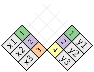
A join is a way of connecting each row in
xto zero, one, or more rows iny.
The following diagram shows each potential match as an intersection of a pair of lines.
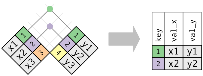
In an actual join, matches will be indicated with dots. The number of dots = the number of matches = the number of rows in the output.
Inner join
An inner join matches pairs of observations whenever their keys are equal

The output of an inner join is a new data frame that contains the
key, the x values, and the y values. We use by to tell
dplyr which variable is the key:
x %>%
  inner_join(y, by = "key")
## # A tibble: 2 × 3
## key val_x val_y
## <dbl> <chr> <chr>
## 1 1 x1 y1
## 2 2 x2 y2The most important property of an inner join is that unmatched rows are not included in the result.
This means that generally inner joins are usually not appropriate for use in analysis because

Its too easy to lose observations
Outer joins
An outer join keeps observations that appear in at least one of the tables.
There are three types of outer joins:
| Join | Action |
|---|---|
| left | keeps all observations in x. |
| right | keeps all observations in y. |
| full | keeps all observations in x and
y. |
These joins work by adding an additional “virtual” observation to
each table. This observation has a key that always matches (if no other
key matches), and a value filled with NA.
Graphically, that looks like:
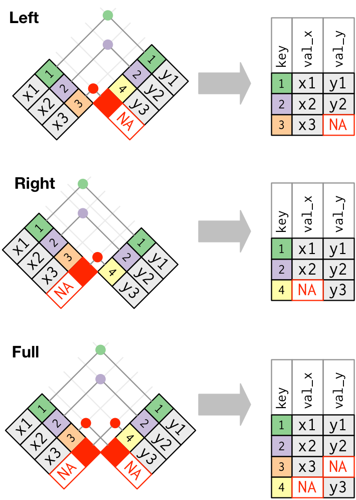
The most commonly used join is the left join.
In summary
Another way to depict the different types of joins is with a Venn diagram:

Duplicate keys
So far all the diagrams have assumed that the keys are unique. But that’s not always the case. There are two possibilities:
One table has duplicate keys.
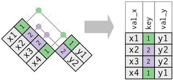
x <- tribble(
  ~key, ~val_x,
     1, "x1",
     2, "x2",
     2, "x3",
     1, "x4"
)
y <- tribble(
  ~key, ~val_y,
     1, "y1",
     2, "y2"
)
left_join(x, y, by = "key")
## # A tibble: 4 × 3 ## key val_x val_y ## <dbl> <chr> <chr> ## 1 1 x1 y1 ## 2 2 x2 y2 ## 3 2 x3 y2 ## 4 1 x4 y1Both tables have duplicate keys. This is usually an ERROR because in neither tables the keys uniquely identify an observation. When you join duplicated keys, you get all possible combinations, the Cartesian product:
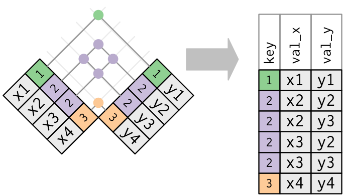
x <- tribble(
  ~key, ~val_x,
     1, "x1",
     2, "x2",
     2, "x3",
     3, "x4"
)
y <- tribble(
  ~key, ~val_y,
     1, "y1",
     2, "y2",
     2, "y3",
     3, "y4"
)
left_join(x, y, by = "key")
## # A tibble: 6 × 3 ## key val_x val_y ## <dbl> <chr> <chr> ## 1 1 x1 y1 ## 2 2 x2 y2 ## 3 2 x2 y3 ## 4 2 x3 y2 ## 5 2 x3 y3 ## 6 3 x4 y4
Defining the key columns
You can use other values for by to connect the
tables in other ways:
The default,
by = NULL, uses all variables that appear in both tables, the so called natural join. For example, the flights and weather tables match on their common variables:year,month,day,hourandorigin.flights2 %>% left_join(weather)## Joining, by = c("year", "month", "day", "hour", "origin")## # A tibble: 336,776 × 18 ## year month day hour origin dest tailnum carrier temp dewp humid wind_dir ## <int> <int> <int> <dbl> <chr> <chr> <chr> <chr> <dbl> <dbl> <dbl> <dbl> ## 1 2013 1 1 5 EWR IAH N14228 UA 39.0 28.0 64.4 260 ## 2 2013 1 1 5 LGA IAH N24211 UA 39.9 25.0 54.8 250 ## 3 2013 1 1 5 JFK MIA N619AA AA 39.0 27.0 61.6 260 ## 4 2013 1 1 5 JFK BQN N804JB B6 39.0 27.0 61.6 260 ## 5 2013 1 1 6 LGA ATL N668DN DL 39.9 25.0 54.8 260 ## 6 2013 1 1 5 EWR ORD N39463 UA 39.0 28.0 64.4 260 ## 7 2013 1 1 6 EWR FLL N516JB B6 37.9 28.0 67.2 240 ## 8 2013 1 1 6 LGA IAD N829AS EV 39.9 25.0 54.8 260 ## 9 2013 1 1 6 JFK MCO N593JB B6 37.9 27.0 64.3 260 ## 10 2013 1 1 6 LGA ORD N3ALAA AA 39.9 25.0 54.8 260 ## # … with 336,766 more rows, and 6 more variables: wind_speed <dbl>, wind_gust <dbl>, ## # precip <dbl>, pressure <dbl>, visib <dbl>, time_hour <dttm>
A character vector,
by = "x". This is like a natural join, but uses only some of the common variables. For example,flightsandplaneshaveyearvariables, but they mean different things so we only want to join bytailnum.flights2 %>% left_join(planes, by = "tailnum")## # A tibble: 336,776 × 16 ## year.x month day hour origin dest tailnum carrier year.y type manufacturer model ## <int> <int> <int> <dbl> <chr> <chr> <chr> <chr> <int> <chr> <chr> <chr> ## 1 2013 1 1 5 EWR IAH N14228 UA 1999 Fixed w… BOEING 737-… ## 2 2013 1 1 5 LGA IAH N24211 UA 1998 Fixed w… BOEING 737-… ## 3 2013 1 1 5 JFK MIA N619AA AA 1990 Fixed w… BOEING 757-… ## 4 2013 1 1 5 JFK BQN N804JB B6 2012 Fixed w… AIRBUS A320… ## 5 2013 1 1 6 LGA ATL N668DN DL 1991 Fixed w… BOEING 757-… ## 6 2013 1 1 5 EWR ORD N39463 UA 2012 Fixed w… BOEING 737-… ## 7 2013 1 1 6 EWR FLL N516JB B6 2000 Fixed w… AIRBUS INDU… A320… ## 8 2013 1 1 6 LGA IAD N829AS EV 1998 Fixed w… CANADAIR CL-6… ## 9 2013 1 1 6 JFK MCO N593JB B6 2004 Fixed w… AIRBUS A320… ## 10 2013 1 1 6 LGA ORD N3ALAA AA NA <NA> <NA> <NA> ## # … with 336,766 more rows, and 4 more variables: engines <int>, seats <int>, speed <int>, ## # engine <chr>Note that the
yearvariables (which appear in both input data frames, but are not constrained to be equal) are disambiguated in the output with a suffix.
A named character vector:
by = c("a" = "b"). This will match variableain tablexto variablebin tabley. The variables fromxwill be used in the output.For example, if we want to draw a map we need to combine the flights data with the airports data which contains the location (
latandlong) of each airport. Each flight has an origin and destinationairport, so we need to specify which one we want to join to:flights2 %>% left_join(airports, c("dest" = "faa"))## # A tibble: 336,776 × 15 ## year month day hour origin dest tailnum carrier name lat lon alt tz dst ## <int> <int> <int> <dbl> <chr> <chr> <chr> <chr> <chr> <dbl> <dbl> <dbl> <dbl> <chr> ## 1 2013 1 1 5 EWR IAH N14228 UA Geor… 30.0 -95.3 97 -6 A ## 2 2013 1 1 5 LGA IAH N24211 UA Geor… 30.0 -95.3 97 -6 A ## 3 2013 1 1 5 JFK MIA N619AA AA Miam… 25.8 -80.3 8 -5 A ## 4 2013 1 1 5 JFK BQN N804JB B6 <NA> NA NA NA NA <NA> ## 5 2013 1 1 6 LGA ATL N668DN DL Hart… 33.6 -84.4 1026 -5 A ## 6 2013 1 1 5 EWR ORD N39463 UA Chic… 42.0 -87.9 668 -6 A ## 7 2013 1 1 6 EWR FLL N516JB B6 Fort… 26.1 -80.2 9 -5 A ## 8 2013 1 1 6 LGA IAD N829AS EV Wash… 38.9 -77.5 313 -5 A ## 9 2013 1 1 6 JFK MCO N593JB B6 Orla… 28.4 -81.3 96 -5 A ## 10 2013 1 1 6 LGA ORD N3ALAA AA Chic… 42.0 -87.9 668 -6 A ## # … with 336,766 more rows, and 1 more variable: tzone <chr>flights2 %>% left_join(airports, c("origin" = "faa"))## # A tibble: 336,776 × 15 ## year month day hour origin dest tailnum carrier name lat lon alt tz dst ## <int> <int> <int> <dbl> <chr> <chr> <chr> <chr> <chr> <dbl> <dbl> <dbl> <dbl> <chr> ## 1 2013 1 1 5 EWR IAH N14228 UA Newa… 40.7 -74.2 18 -5 A ## 2 2013 1 1 5 LGA IAH N24211 UA La G… 40.8 -73.9 22 -5 A ## 3 2013 1 1 5 JFK MIA N619AA AA John… 40.6 -73.8 13 -5 A ## 4 2013 1 1 5 JFK BQN N804JB B6 John… 40.6 -73.8 13 -5 A ## 5 2013 1 1 6 LGA ATL N668DN DL La G… 40.8 -73.9 22 -5 A ## 6 2013 1 1 5 EWR ORD N39463 UA Newa… 40.7 -74.2 18 -5 A ## 7 2013 1 1 6 EWR FLL N516JB B6 Newa… 40.7 -74.2 18 -5 A ## 8 2013 1 1 6 LGA IAD N829AS EV La G… 40.8 -73.9 22 -5 A ## 9 2013 1 1 6 JFK MCO N593JB B6 John… 40.6 -73.8 13 -5 A ## 10 2013 1 1 6 LGA ORD N3ALAA AA La G… 40.8 -73.9 22 -5 A ## # … with 336,766 more rows, and 1 more variable: tzone <chr>
Another implementation of Joins
base::merge() can perform all four types of mutating
join:
| dplyr | merge |
|---|---|
inner_join(x, y) |
merge(x, y) |
left_join(x, y) |
merge(x, y, all.x = TRUE) |
right_join(x, y) |
merge(x, y, all.y = TRUE), |
full_join(x, y) |
merge(x, y, all.x = TRUE, all.y = TRUE) |
The advantages of the specific dplyr verbs is that they more clearly
convey the intent of your code: the difference between the joins is
really important but concealed in the arguments of merge().
dplyr’s joins are considerably faster and don’t mess with the order of
the rows.
Filtering joins

Filtering joins match observations in the same way as mutating joins, but affect the observations, not the variables.
There are two types:
| Join | Action |
|---|---|
semi_join(x, y) |
keeps all observations in x that have
a match in y. |
anti_join(x, y) |
drops all observations in x that have
a match in y. |
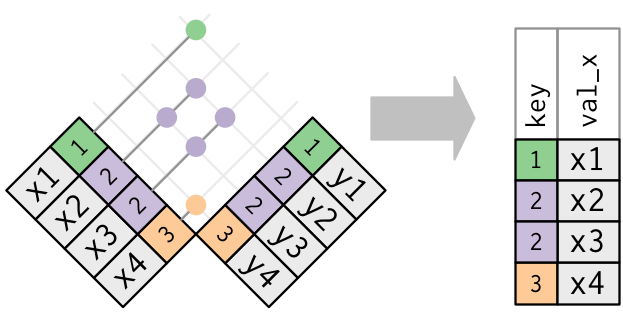
Graphically, a semi-join looks like this:
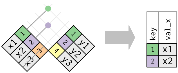
Only the existence of a match is important
it doesn’t matter which observation is matched. This means that filtering joins never duplicate rows like mutating joins do:
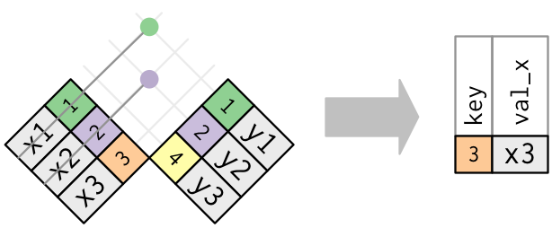
The inverse of a semi-join is an anti-join.
An anti-join keeps the rows that don’t have a match:
Set operations
The final type of two-table verb are the set operations.
All these operations work with a complete row, comparing the values
of every variable. These expect the x and y
inputs to have the same variables, and treat the observations like
sets:
intersect(x, y): return only observations in bothxandy.union(x, y): return unique observations inxandy.setdiff(x, y): return observations inx, but not iny.
Given this simple data:
df1 <- tribble(
  ~x, ~y,
   1,  1,
   2,  1
)
df2 <- tribble(
  ~x, ~y,
   1,  1,
   1,  2
)
The four possibilities are:
intersect(df1, df2)## # A tibble: 1 × 2
## x y
## <dbl> <dbl>
## 1 1 1# Note that we get 3 rows, not 4
union(df1, df2)## # A tibble: 3 × 2
## x y
## <dbl> <dbl>
## 1 1 1
## 2 2 1
## 3 1 2setdiff(df1, df2)## # A tibble: 1 × 2
## x y
## <dbl> <dbl>
## 1 2 1setdiff(df2, df1)## # A tibble: 1 × 2
## x y
## <dbl> <dbl>
## 1 1 2A work by Matteo Cereda and Fabio Iannelli